---
title: 2 · Steady-state RANS
section: tutorials
order: 20
---
# Steady-state RANS
## What is in this tutorial?
[Simple aerofoil](./1-simple-aerofoil.md) showed how to run a case in zCFD and look at the results. This tutorial
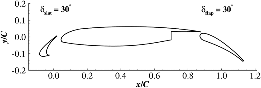
uses a harder case to show more of the solver: the 30P30N, a high-lift aerofoil of the kind a wing uses for take-off
and landing. It has three parts: a slat at the front, the main element, and a flap at the back, with gaps between
them. It is a well-known test case, first developed to study the noise these wings make [[1]](#citations).
You run it at an angle of attack, the angle between the oncoming flow and the aerofoil's chord, and report the lift
(the force across the flow) and the drag (the force along it). The first run stops before the answer has settled, so
you then restart it from where it stopped and carry it on.
## What you need?
Work through [Simple aerofoil](./1-simple-aerofoil.md) first: this tutorial relies on it for activating zCFD,
running a case and reading its output. The case has 64,000 cells. On an NVIDIA RTX 3060 the
first run takes under two minutes and the restart about a minute.
::: {.track when="deck"}
## Step 1. Download the files
The tutorial bundle can be downloaded [here](https://zcfd.zenotech.com/v2026.11.16174/tutorial_2_high_lift_multi_element_aerofoil.tgz).
It contains a mesh file (`30p30n.h5`) and a zCFD control file (`30p30n.py`).
```bash
cd ~
wget https://zcfd.zenotech.com/v2026.11.16174/tutorial_2_high_lift_multi_element_aerofoil.tgz
tar xzf tutorial_2_high_lift_multi_element_aerofoil.tgz
cd tutorial_2_high_lift_multi_element_aerofoil
```
## Step 2. Walk through the input
The control file, `30p30n.py`, is a short Python script. All it does is build one Python dictionary, called
`parameters`, that tells zCFD everything about the run: the physics, the numerical method, what to write out, and
the mesh with its boundaries. This step walks through that dictionary from top to bottom. Each heading below is the
name of a key, written exactly as it appears in the file, and the headings nest the same way the dictionary does:
`numerical scheme`, for example, sits inside `solver`. Under each heading you'll find what that part controls, what
each setting means, and why it has the value it has here. Each section ends with a link to that part's reference
page, which lists every setting it accepts and its default; you don't need it to follow the tutorial. On a wide
screen the whole control file sits on the right, with the part being described highlighted as you scroll.
```python
import math
import zutil
reynolds = 1.71e6
mach = 0.17
T = 295.56
p = 101325
R = 287.6
gamma = 1.4
reference_length = 0.457
alpha = 5.5
U = math.sqrt(gamma * R * T) * mach
wall = [6]
symmetry = [4, 5]
farfield = [7]
def my_transform(*, vector):
return zutil.rotate_vector(vector, alpha, 0.0)
parameters = {
"config version": 2,
"solver": {
"solver settings": {"type": "compressible"},
"equations": {
"type": "rans",
"turbulence": {
"model": "sst",
"limit mut": False,
"production": "strain-compressible",
},
"precondition": True,
},
"fluid properties": {
"material": "air",
"gamma": gamma,
"gas constant": R,
"sutherlands const": 110.4,
"prandtl no": 0.72,
"turbulent prandtl no": 0.9,
},
"reference conditions": {
"IC_1": {
"temperature": T,
"pressure": p,
"v": {"vector": zutil.vector_from_angle(alpha, 0.0, U)},
"reynolds no": reynolds,
"reference length": reference_length,
"turbulence intensity": 0.01,
"eddy viscosity ratio": 0.1,
},
},
"initialisation": {"initial conditions": "IC_1", "restart": False},
"numerical scheme": {
"order": "euler_second",
"inviscid flux scheme": "roe",
},
"time settings": {"type": "steady"},
"convergence control": {
"scheme": {"name": "implicit euler"},
"cfl": {
"cfl": 50.0,
"cfl ramp": [{"type": "exponential", "factor": 1.1, "initial": 1.0}],
},
"cycles": 1000,
},
"output settings": {
"report": {
"frequency": 50,
"forces": {
"FR_1": {
"name": "wall",
"zones": wall,
"transform": my_transform,
"reference area": 0.4572,
},
},
},
"solution": {
"frequency": 500,
"surface variables": ["p", "cp", "V"],
"volume variables": [
"V",
"p",
"T",
"rho",
"var_6",
"eddy",
"turbulencekineticenergy",
"turbulenceeddyfrequency",
"walldist",
],
},
},
},
"model": {
"30p30n": {
"mesh": "30p30n.h5",
"transforms": {"scale": [0.0254, 0.0254 / 0.127, 0.0254]},
"boundary conditions": {
"BC_1": {"zones": symmetry, "type": "symmetry"},
"BC_2": {"zones": wall, "type": "wall", "kind": "no slip"},
"BC_3": {
"zones": farfield,
"type": "farfield",
"condition": "IC_1",
"kind": "riemann",
},
},
},
},
}
```
Unlike the first tutorial's file, this one runs a little ordinary Python before the dictionary, to set the flow
conditions once and work out values from them. The first two headings cover that code.
### `reynolds`, `mach`, `T`, `p`, `R`, `gamma`, `reference_length`, `alpha`, `U`, `wall`, `symmetry`, `farfield`
The control file is Python, so it can do more than list settings. After importing `math` and `zutil`, its first
lines set the key values for the case once, by name, and the dictionary refers to them:
- `reynolds`: 1.71 million, the Reynolds number based on the chord: how strongly the flow's momentum outweighs its
viscosity.
- `mach`: 0.17, the freestream Mach number: the flow speed as a fraction of the speed of sound.
- `T` and `p`: 295.56 K and 101325 Pa, the freestream temperature and pressure.
- `R` and `gamma`: the gas constant, 287.6 J/kg/K, and the ratio of specific heats, 1.4.
- `reference_length`: 0.457 m, the aerofoil's chord, which the Reynolds number is based on.
- `alpha`: 5.5°, the angle of attack.
- `U`: the freestream speed, worked out from the Mach number and the speed of sound, $\sqrt{\gamma R T}$: 58.6 m/s.
- `wall`, `symmetry` and `farfield`: the mesh zones that the forces and boundary conditions use.
To run a variation of the case, change one value here, and every setting that uses it follows.
### `my_transform`
A function that turns a force from the mesh's axes into the flow's. Lift and drag are defined relative to the
freestream, lift normal to it and drag along it. `zutil.rotate_vector(vector, alpha, 0.0)` rotates a vector through
the angle of attack, so that its x component is the drag and its z component the lift. The force report below
applies it.
### `config version`
The version of the control-file format. `2` is the current format.
### `solver`
Everything shared by the whole simulation.
#### `solver settings`
Which solver runs the case. [Reference](/reference/solver/solver-settings).
- `type`: `"compressible"`, the density-based solver.
#### `equations`
Which equations are solved. [Reference](/reference/solver/equations).
- `type`: `"rans"`, the Reynolds-averaged Navier–Stokes equations, which solve for the average flow and use a
turbulence model for the effect of turbulent eddies, as in [Simple aerofoil](./1-simple-aerofoil.md#equations).
- `turbulence`: the turbulence model and its options.
- `model`: `"sst"`, Menter's SST model. The mesh is fine enough next to the surfaces to resolve the boundary
layer all the way down to the wall.
- `limit mut`: `False` switches off the SST model's limit on the eddy viscosity, which is on by default. The eddy
viscosity is the extra viscosity the turbulence model adds to represent the mixing done by turbulent eddies.
- `production`: `"strain-compressible"` sets how the model works out how fast turbulence is generated: from how
quickly the flow is being stretched (the strain rate), instead of the default, from how fast it is spinning (the
vorticity).
- `precondition`: `True` switches on low-Mach-number preconditioning, recommended below about Mach 0.3.
[Choosing a turbulence model](../guide/choosing/choosing-a-turbulence-model.md) compares the models and options.
#### `fluid properties`
The gas the flow is made of. [Reference](/reference/solver/fluid-properties).
- `material`: `"air"`.
- `gamma` and `gas constant`: taken from the reference variables.
- `sutherlands const`: 110.4 K, for Sutherland's law of viscosity.
- `prandtl no` and `turbulent prandtl no`: 0.72 and 0.9, which relate heat conduction to viscosity in the laminar
flow and the turbulence.
#### `reference conditions`
Named flow states, which the initialisation and the boundary conditions refer to.
[Reference](/reference/solver/reference-conditions).
##### `IC_1`
The freestream, built from the reference variables.
- `temperature` and `pressure`: 295.56 K and 101325 Pa.
- `v`: the velocity. Its `vector` comes from `zutil.vector_from_angle(alpha, beta, U)`, which gives the velocity for
an angle of attack `alpha` and a sideslip `beta`, in degrees, at speed `U`. Following the ESDU convention for
aerodynamic axes, the angle of attack turns the flow from x towards z, so the flow meets the aerofoil at 5.5°, with
no sideslip. The aerofoil stays where it is in the mesh, and the flow is turned instead.
- `reynolds no` and `reference length`: a Reynolds number of 1.71 million on the 0.457 m chord. zCFD works out the
viscosity from them.
- `turbulence intensity`: 0.01, so the velocity fluctuations in the incoming flow are 1% of its speed.
- `eddy viscosity ratio`: 0.1, the ratio of eddy viscosity to molecular viscosity in the incoming flow. Together
with the intensity, it sets the turbulence the SST model starts from.
#### `initialisation`
How the flow field starts. [Reference](/reference/solver/initialisation).
- `initial conditions`: `"IC_1"`, the freestream everywhere.
- `restart`: `False`, a fresh start. Step 3 turns it on to carry the run on.
#### `numerical scheme`
How the equations are discretised in space. [Reference](/reference/solver/numerical-scheme).
- `order`: `"euler_second"`, second order for the flow variables and first order for the turbulence variables,
with the default limiter, as in [Simple aerofoil](./1-simple-aerofoil.md#numerical-scheme).
- `inviscid flux scheme`: `"roe"`, Roe's scheme for the flow between cells.
#### `time settings`
[Reference](/reference/solver/time-settings).
- `type`: `"steady"`, a solution that does not change with time.
#### `convergence control`
How the solver marches towards the steady solution, once per cycle. [Reference](/reference/solver/convergence-control).
- `scheme`: `implicit euler`, which solves a linear system each cycle and allows large steps.
- `cfl`: the CFL number ramps from 1 by a factor of 1.1 each cycle up to 50.
- `cycles`: 1000. As Step 4 shows, that is not quite enough, and Step 3 carries the run on with a restart.
#### `output settings`
What zCFD writes, and how often. [Reference](/reference/solver/output-settings).
##### `report`
The report is the CSV file `30p30n_report.csv`: one row of residuals and forces at a time, which zMon plots.
- `frequency`: 50, a row every 50 cycles.
- `forces`: force blocks, each summing the pressure and friction forces on a set of zones. This deck has one,
`FR_1`:
- `name`: `"wall"`. The report names the block's columns after it: `wall_Fx`, `wall_Fy` and `wall_Fz` are the
forces in mesh axes, split into pressure (`wall_Fpx`, ...) and friction (`wall_Ffx`, ...) parts, and
`wall_Mx` and so on are the moments.
- `zones`: the `wall` zones from the top of the file, zone 6: the slat, main element and flap together.
- `transform`: `my_transform`. The report gains the transformed forces and moments, in columns starting
`wall_Ft` and `wall_Mt`: `wall_Ftx` is the drag and `wall_Ftz` the lift.
- `reference area`: 0.4572 m², the chord times the 1 m span. Forces are reported as coefficients against `IC_1`
and this area, so `wall_Ftx` and `wall_Ftz` are the drag and lift coefficients.
##### `solution`
The flow fields written for viewing in ParaView.
- `frequency`: 500. In a steady run, zCFD writes the fields every 500 cycles, each time replacing the last, so a
run that stops early still leaves a recent solution.
- `surface variables`: on the boundaries: pressure `p`, pressure coefficient `cp` and velocity `V`.
- `volume variables`: in every cell: velocity, pressure, temperature and density, the sixth solved variable `var_6`
($\rho k$), the eddy viscosity `eddy`, the turbulence kinetic energy and eddy frequency, and `walldist`, the distance to
the nearest wall, which the SST model uses.
[Output variables](../guide/working-with/post-processing-and-visualisation.md#output-variables) lists every variable.
### `model`
One entry per mesh, each with its own boundary conditions. [Reference](/reference/model).
#### `30p30n`
The only model. Its name, `30p30n`, names its output folder, `30p30n_OUTPUT/30p30n/`, and its output files.
##### `mesh`
- `"30p30n.h5"`, a zCFD mesh with 64,000 cells and a single cell across the span. It follows the ESDU convention for
aerodynamic axes: x points downstream along the chord, z points up and y runs along the span. It was built in
inches.
##### `transforms`
Changes made to the mesh as it is read, without editing the file. [Reference](/reference/model/transforms).
- `scale`: multiplies the x, y and z coordinates of the file. 0.0254 turns inches into metres. The y factor,
0.0254 / 0.127, stretches the 5 inch span to 1 m: there is no spanwise flow, and a 1 m span makes the reported
forces per unit span.
[Placing and moving a mesh](../guide/working-with/placing-and-moving-a-mesh.md) describes the other ways to place a
mesh.
##### `boundary conditions`
A condition for each group of boundary faces, named by the zone lists at the top of the file.
[Choosing boundary conditions](../guide/choosing/choosing-boundary-conditions.md) describes every type.
###### `BC_1`
- `zones`: `symmetry`, zones 4 and 5, the two faces normal to the span.
- `type`: `"symmetry"`, so the flow behaves as if the aerofoil were infinitely long and stays 2D.
###### `BC_2`
- `zones`: `wall`, zone 6, the surfaces of the slat, main element and flap.
- `type`: `"wall"`, with `kind` `"no slip"`: the flow velocity is zero at the surface.
###### `BC_3`
- `zones`: `farfield`, zone 7, the outer boundary.
- `type`: `"farfield"`, with `condition` `"IC_1"`, the freestream outside.
- `kind`: `"riemann"`, which passes waves out without reflecting them back into the domain.
## Step 3. Run
Activate zCFD as in [Simple aerofoil](./1-simple-aerofoil.md#step-3-run), then check and run the case:
```bash
cd ~/tutorial_2_high_lift_multi_element_aerofoil/
validate_input 30p30n.py
run_zcfd -c 30p30n.py
```
These are extracts from the log of a run of this tutorial, with `...` marking lines left out:
```text
Parameters validated successfully
...
Reading file 30p30n.h5
Global Mesh Stats: Cells: 63957 Faces: 256413
...
Viscosity: 1.86824e-05 Ns/m^2 @ 295.56 K
Speed: 58.6449 m/s
...
Mach: 0.17
Reynolds No: 1.71e+06 @ 295.56 K
...
Starting solve loop
...
Cycle 50 | Step 0 t=0s | CFL 50.000 | MG 1 | 39.9 ms | Total 1.328s
+------------------------------------------------------------------------------------------+
| Report: Cycle 50 Wall time: 1.328s |
...
| Residuals: |
| rho 5.0013E-01 rhoV[0] 1.0090E+00 rhoV[1] 1.7333E-11 rhoV[2] 8.5874E-01 |
| rhoE 1.7070E+00 rhok 4.4082E-07 rhoOmega 1.4652E+05 |
+------------------------------------------------------------------------------------------+
...
Solve Complete: 1000 cycles in 36.943s (avg 36.9 ms/cycle)
...
zCFD finished: all requested cycles are complete (1000 in total).
```
The lines are the same as in the first tutorial. The viscosity is worked out from the Reynolds number, and the
speed, 58.6 m/s, from the Mach number. In the report box every 50 cycles, `rhoV[1]`, the momentum along the span (y),
stays below 10-10: with a single cell across the span, no flow develops in that direction.
### Restarting the run
Step 4 shows that after 1000 cycles the residuals are still falling. Rather than start again, restart the run from
where it stopped. In `30p30n.py`, turn on `restart` under `initialisation`, and raise `cycles` under
`convergence control` to 2000, the total the run should reach:
```python
"initialisation": {"initial conditions": "IC_1", "restart": True},
```
```python
"cycles": 2000,
```
With `restart` on, zCFD reads the checkpoint the previous run of the same control file wrote,
`30p30n_OUTPUT/30p30n/30p30n_results.h5`, and carries on from cycle 1001. Run it with the same command:
```bash
run_zcfd -c 30p30n.py
```
The log says where it restarted from:
```text
Restarting solution from results file 30p30n_OUTPUT/30p30n/30p30n
...
Cycle 1001 | Step 0 t=0s | CFL 1.100 | MG 1 | 97.1 ms | Total 0.097s
...
Cycle 2000 | Step 0 t=0s | CFL 50.000 | MG 1 | 23.1 ms | Total 25.001s
+------------------------------------------------------------------------------------------+
| Report: Cycle 2000 Wall time: 25.001s |
...
| Residuals: |
| rho 4.4183E-04 rhoV[0] 5.1424E-03 rhoV[1] 1.6681E-14 rhoV[2] 1.3771E-03 |
| rhoE 1.0785E-03 rhok 8.6709E-06 rhoOmega 1.5141E+03 |
+------------------------------------------------------------------------------------------+
...
zCFD finished: all requested cycles are complete (2000 in total).
```
The CFL ramp starts again from its initial value, so the first restarted cycles take small steps.
[Choosing initialisation and reference state](../guide/choosing/choosing-initialisation-and-reference-state.md)
covers restarts in full.
### Output files
The output follows the same pattern as the first tutorial, named after the control file and the model. The
restarted run appends to the same report.
| File/Directory | Description |
| --------------------------------------------- | ---------------------------------------------------------------------------------- |
| `30p30n.log` | A copy of the output to screen during the run. |
| `30p30n_status.yaml` | A YAML file recording how the run was started. |
| `30p30n_OUTPUT/30p30n/30p30n_report.csv` | The report: residuals and forces, including the `wall_Ftx` and `wall_Ftz` columns. |
| `30p30n_OUTPUT/30p30n/30p30n_results.h5` | The checkpoint, which the restart reads. |
| `30p30n_OUTPUT/30p30n/30p30n.vtkhdf` | The volume data. |
| `30p30n_OUTPUT/30p30n/30p30n_wall.vtkhdf` etc | One file for each boundary condition type, with the surface data. |
## Step 4. Monitor
Open the case in zMon to follow the residuals and forces as the solver runs:
```bash
zmon 30p30n.py
```
zMon follows the restarted run too, which appends to the same report. The plots below are the
panels as zMon draws them; [Step 5](#step-5-post-process) shows how to plot the same data yourself.
### Residuals
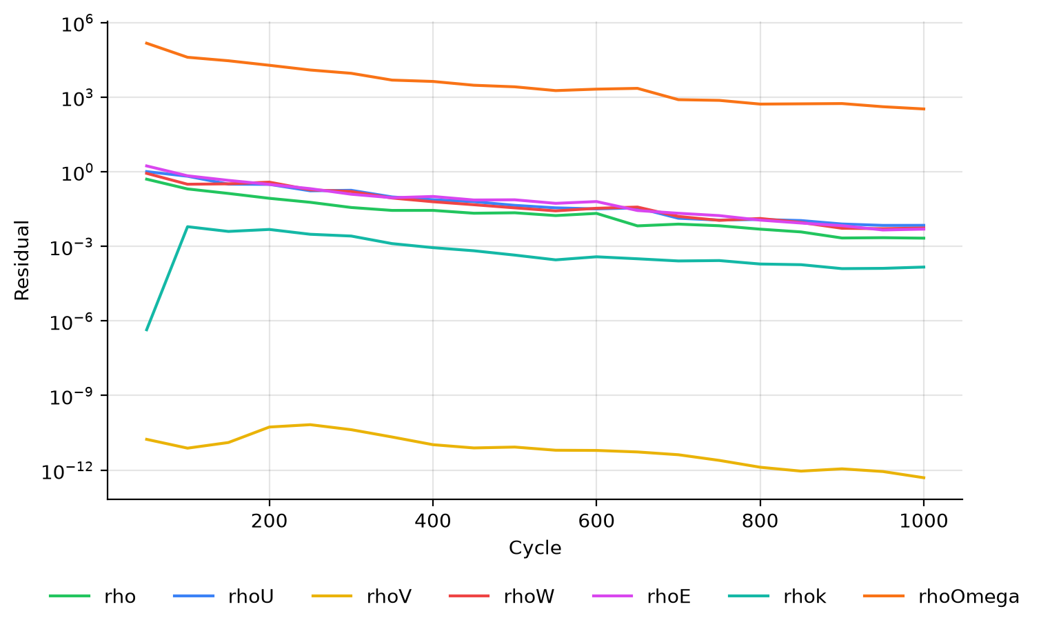
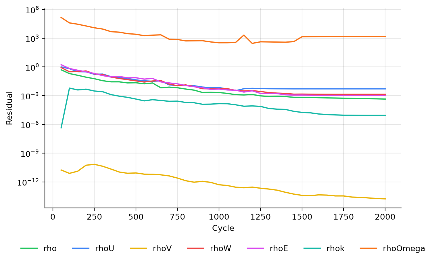
After the first 1000 cycles the residuals are still falling, which is why the run is restarted. By the end of the
restarted run they have levelled off:
### Forces
The forces of interest are the transformed ones, `wall_Ftx` (drag) and `wall_Ftz` (lift), in zMon's forces panel:
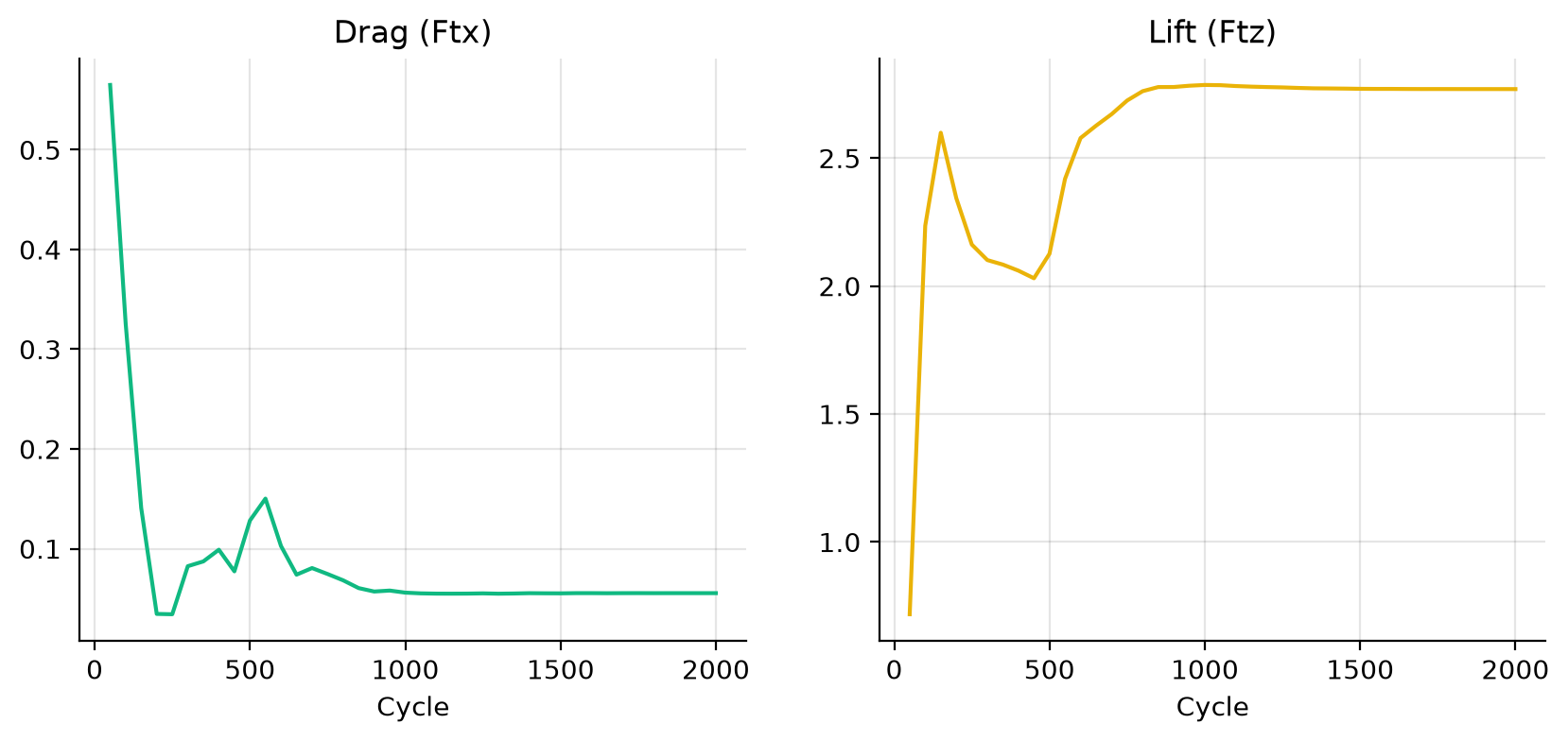
Both have converged by the end of the restarted run, with a lift coefficient of 2.77 and a drag coefficient of
0.055. The grid for this case is still extremely coarse, so these lift and drag coefficients are not a validation
of the 30P30N.
## Step 5. Post-process
First activate your zCFD environment, which provides Python with zutil, h5py and ParaView:
```bash
source /bin/activate
```
### Python
This script draws the plots in [Step 4](#step-4-monitor) and prints the final lift and drag coefficients. It is the
first tutorial's script with the transformed force columns, `wall_Ftx` and `wall_Ftz`. Save it as
`plot_convergence.py` in the case directory:
```python
import matplotlib.pyplot as plt
from zutil.fileutils import get_zcfd_result
report = get_zcfd_result("30p30n.py").report.data
fig, ax = plt.subplots()
for column in ["rho", "rhoV[0]", "rhoV[1]", "rhoV[2]", "rhoE", "rhok", "rhoOmega"]:
ax.semilogy(report["Cycle"], report[column], label=column)
ax.set_xlabel("Cycle")
ax.set_ylabel("Residual")
ax.legend()
fig.savefig("residuals.png", dpi=200)
fig, (drag, lift) = plt.subplots(1, 2, figsize=(10, 4))
drag.plot(report["Cycle"], report["wall_Ftx"])
drag.set_title("Drag coefficient (wall_Ftx)")
lift.plot(report["Cycle"], report["wall_Ftz"])
lift.set_title("Lift coefficient (wall_Ftz)")
for ax in (drag, lift):
ax.set_xlabel("Cycle")
fig.savefig("forces.png", dpi=200)
final = report.iloc[-1]
print(f"Lift coefficient {final['wall_Ftz']:.2f}, drag coefficient {final['wall_Ftx']:.3f}")
```
Run it:
```bash
python plot_convergence.py
```
It writes `residuals.png` and `forces.png`, and prints:
```text
Lift coefficient 2.77, drag coefficient 0.055
```
### ParaView
Open `30p30n_OUTPUT/30p30n/30p30n_wall.vtkhdf` in ParaView to see the results on the aerofoil surfaces, here
coloured by the pressure coefficient:
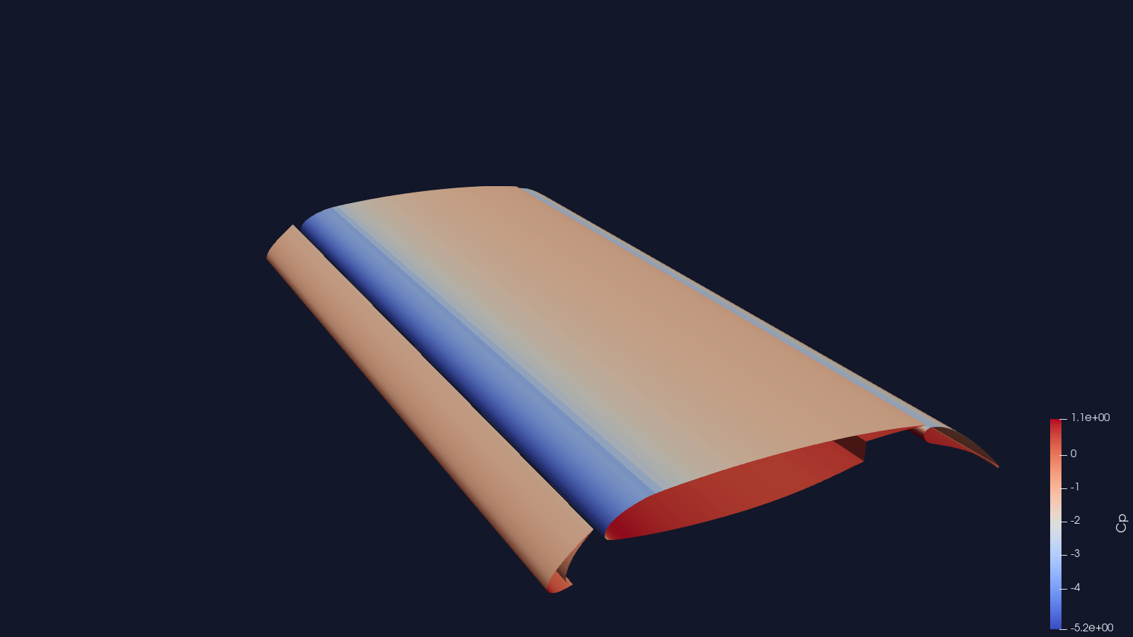
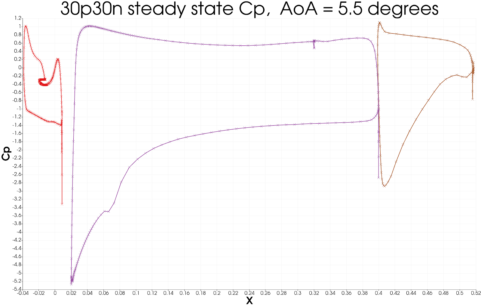
To plot the pressure coefficient along the chord (x/c, the distance from the front divided by the chord), use a
"Plot On Sorted Lines" filter:
1. On the surface data apply a _'cell data to point data'_ filter.
2. On the _cell data to point data_ apply a _'slice'_ filter, ensuring the slice uses a y normal, and is centred
through the middle of the span.
3. On the _slice_ data apply a _'plot on sorted lines'_ filter and click apply. This will then bring up a new
_'line graph'_ view.
4. Ensure all 3 segments are selected in the composite data set dialogue box, then ensure only the cp variables
are selected in the series parameters. Finally for the X Array name, select `Points_X`
5. Modify the style and markers until you are happy with the result.
:::
## Citations
1. Zhang, Yufei & Chen, Haixin & Wang, Kan & Wang, Meng. (2017). Aeroacoustic Prediction of a Multi-Element
Airfoil Using Wall-Modeled Large-Eddy Simulation. AIAA Journal. 55. 1-15. 10.2514/1.J055853.