---
title: 3 · Time-accurate solution
section: tutorials
order: 30
---
# Time-accurate solution
## What is in this tutorial?
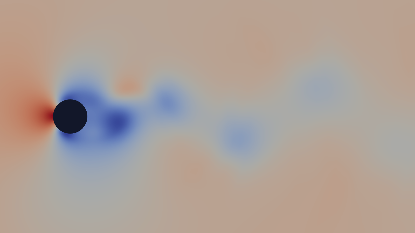
Some flows never settle to a steady state. Behind a cylinder, swirling vortices peel off each side in turn and are
carried away downstream, and the flow repeats over and over at a definite frequency. This is vortex shedding, the
same effect that makes wires hum in the wind.
The previous tutorials looked for a steady answer. Here the answer changes with time, so the run has to follow it
step by step in real time: a time-accurate run. The flow is a cylinder in a slow, smooth (laminar) flow at a
Reynolds number of 150. You record the pressure at one point in the wake and measure the shedding frequency from
it.
## What you need?
Work through [Simple aerofoil](./1-simple-aerofoil.md) first: this tutorial relies on it for activating zCFD,
running a case and reading its output. The run takes about four minutes on an NVIDIA RTX 3060.
::: {.track when="deck"}
## Step 1. Download the files
The tutorial bundle can be downloaded [here](https://zcfd.zenotech.com/v2026.11.16174/tutorial_3_cylinder_shedding.tgz).
It contains a mesh file (`cylinder.h5`) and a zCFD control file (`cylinder.py`).
```bash
cd ~
wget https://zcfd.zenotech.com/v2026.11.16174/tutorial_3_cylinder_shedding.tgz
tar xzf tutorial_3_cylinder_shedding.tgz
cd tutorial_3_cylinder_shedding
```
## Step 2. Walk through the input
The control file, `cylinder.py`, is a short Python script. All it does is build one Python dictionary, called
`parameters`, that tells zCFD everything about the run: the physics, the numerical method, what to write out, and
the mesh with its boundaries. This step walks through that dictionary from top to bottom. Each heading below is the
name of a key, written exactly as it appears in the file, and the headings nest the same way the dictionary does:
`numerical scheme`, for example, sits inside `solver`. Under each heading you'll find what that part controls, what
each setting means, and why it has the value it has here. Each section ends with a link to that part's reference
page, which lists every setting it accepts and its default; you don't need it to follow the tutorial. On a wide
screen the whole control file sits on the right, with the part being described highlighted as you scroll.
```python
parameters = {
"config version": 2,
"solver": {
"solver settings": {"type": "compressible"},
"equations": {
"type": "viscous",
"precondition": True,
},
"fluid properties": {
"material": "air",
"gamma": 1.4,
"gas constant": 287.0,
"sutherlands const": 110.4,
"prandtl no": 0.72,
},
"reference conditions": {
"IC_1": {
"temperature": 277.7777,
"pressure": 101325.0,
"v": {"vector": [0.0, 1.0, 0.0], "mach": 0.2},
"reynolds no": 150,
"reference length": 1.0,
},
},
"initialisation": {"initial conditions": "IC_1", "restart": False},
"numerical scheme": {
"order": "second",
"inviscid flux scheme": "roe",
},
"time settings": {
"type": "unsteady",
"kind": "dual time stepping",
"total time": 1.6,
"time step": 0.002,
"order": "second",
"start": 0,
},
"convergence control": {
"scheme": {"name": "implicit euler"},
"cfl": {
"cfl": 200,
"cfl viscous factor": 1.0e-6,
"cfl ramp": [{"type": "exponential", "factor": 1.05, "initial": 0.1}],
},
"cycles": 5,
},
"output settings": {
"report": {
"frequency": 5,
"monitor": {
"MR_1": {
"name": "probe",
"point": [0.25, 1.07, 0.313],
"variables": ["cp"],
},
},
},
"solution": {
"format": "vtk",
"surface variables": ["V", "p", "T", "rho", "cp"],
"volume variables": ["V", "p", "T", "rho", "m", "cp"],
"frequency": {
"volume data": 5,
"surface data": 5,
"checkpoint": 20,
},
},
},
},
"model": {
"cylinder": {
"mesh": "cylinder.h5",
"boundary conditions": {
"BC_1": {"zones": [2], "type": "symmetry"},
"BC_2": {"zones": [3], "type": "wall", "kind": "no slip"},
"BC_3": {
"zones": [1],
"type": "farfield",
"condition": "IC_1",
"kind": "riemann",
},
},
},
},
}
```
If you have worked through [Simple aerofoil](./1-simple-aerofoil.md), the parts that are new here are
`time settings`, `convergence control` and `output settings`.
### `config version`
The version of the control-file format. `2` is the current format, which zCFD checks before it reads anything else.
### `solver`
Everything shared by the whole simulation: the equations, the flow conditions, how the run marches in time and what
it writes.
#### `solver settings`
Which solver runs the case. [Reference](/reference/solver/solver-settings).
- `type`: `"compressible"`, the density-based solver. At Mach 0.2 the flow is nearly incompressible, but the
compressible solver with preconditioning handles it well.
#### `equations`
Which equations are solved. [Reference](/reference/solver/equations).
- `type`: `"viscous"`, the Navier–Stokes equations with no turbulence model. At a Reynolds number of 150 the flow
round the cylinder is laminar: smooth and orderly, apart from the vortices themselves, so no turbulence model is
needed.
- `precondition`: `True` switches on low-Mach-number preconditioning, which keeps the solver efficient and accurate
at low Mach numbers. It is recommended below about Mach 0.3.
#### `fluid properties`
The gas the flow is made of. [Reference](/reference/solver/fluid-properties).
- `material`: `"air"`.
- `gamma`: 1.4, the ratio of specific heats.
- `gas constant`: 287 J/kg/K.
- `sutherlands const`: 110.4 K, the constant in Sutherland's law, which gives the viscosity's change with
temperature.
- `prandtl no`: 0.72, the laminar Prandtl number, which relates heat conduction to viscosity. There is no turbulent
Prandtl number, as there is no turbulence model.
#### `reference conditions`
Named flow states, which the initialisation and the boundary conditions refer to.
[Reference](/reference/solver/reference-conditions).
##### `IC_1`
The freestream.
- `temperature`: 277.78 K.
- `pressure`: 101325 Pa.
- `v`: the velocity, as a direction and a Mach number: Mach 0.2 along y, which is the flow direction in this mesh.
- `reynolds no`: 150. Instead of a viscosity, the state gives a Reynolds number, and zCFD works out the viscosity
that produces it.
- `reference length`: 1 m, the cylinder's diameter, which the Reynolds number is based on.
#### `initialisation`
How the flow field starts. [Reference](/reference/solver/initialisation).
- `initial conditions`: `"IC_1"` fills the domain with the freestream. The uniform start is symmetric, so the wake
takes a while to break symmetry and begin shedding.
- `restart`: `False`, a fresh start rather than a continuation of an earlier run.
[Choosing initialisation and reference state](../guide/choosing/choosing-initialisation-and-reference-state.md)
covers both.
#### `numerical scheme`
How the equations are discretised in space. [Reference](/reference/solver/numerical-scheme).
- `order`: `"second"` reconstructs every flow variable to second order, with the default limiter keeping it free of
overshoots.
- `inviscid flux scheme`: `"roe"`, Roe's scheme for the flow between cells.
[Choosing a spatial scheme](../guide/choosing/choosing-a-spatial-scheme.md) covers both.
#### `time settings`
What kind of run this is, and how it advances in physical time. This is what makes the run time-accurate.
[Reference](/reference/solver/time-settings).
- `type`: `"unsteady"`, a solution that changes with time.
- `kind`: `"dual time stepping"`. The run advances in real (physical) time steps. At each one it has to find the
flow at the new time, and it does that the same way a steady run finds its answer: by repeating cycles, called
inner cycles, that home in on it. The inner cycles march in an artificial time, pseudo-time, that only matters
inside the step. `convergence control`, below, sets that inner loop.
- `total time`: 1.6 s of physical time.
- `time step`: 0.002 s per step, so the run takes 1.6 / 0.002 = 800 time steps. The step must be small enough to
follow the flow's fastest changes; the shedding period here is about 0.09 s, more than 40 steps.
- `order`: `"second"`, a second-order backward difference for the time derivative. The first steps build up to it
from first order.
- `start`: 0, the number of steady cycles to run before time stepping begins. None here: the run marches from the
uniform start straight away.
[Dual time stepping](../guide/choosing/choosing-a-time-marching-scheme.md#dual-time-stepping) describes the options.
#### `convergence control`
The inner pseudo-time loop that converges each physical time step, set just as it sets the whole solve in a steady
run. [Reference](/reference/solver/convergence-control).
##### `scheme`
- `name`: `"implicit euler"`, which takes each pseudo-time step by solving a linear system, allowing large steps.
##### `cfl`
The CFL number sets the size of each pseudo-time step.
- `cfl`: 200, the CFL number the ramp climbs to.
- `cfl viscous factor`: scales the viscous part of each cell's pseudo-time step estimate. At 10-6 it
leaves the convective wave speeds alone to set the step.
- `cfl ramp`: starts at 0.1 and multiplies the CFL by 1.05 each cycle until it reaches 200, so the first cycles,
far from the answer, take small steps.
##### `cycles`
- 5 inner cycles per physical time step, so the run makes 800 × 5 = 4000 cycles in all.
The time step and the number of inner cycles together set the cost and accuracy of the run. Too large a time step,
or too few inner cycles, and the faster unsteady features are lost; too small a step, or too many cycles, and the
run costs more for no gain. Check a new case by repeating it with a smaller time step or more inner cycles, and
making sure the result you care about, here the shedding frequency, does not change.
[CFL control](../guide/choosing/choosing-a-time-marching-scheme.md#cfl-control) describes the ways to set the CFL.
#### `output settings`
What zCFD writes, and how often. There are two kinds of output: the `report`, a table that grows as the run goes,
and the `solution`, flow fields for viewing. [Reference](/reference/solver/output-settings).
##### `report`
The report is the CSV file `cylinder_report.csv`: one row of residuals, and of any forces and monitors, at a time.
zMon plots it as the run goes.
- `frequency`: 5, a row every 5 cycles. With 5 inner cycles per time step, that is one row per time step, at the end
of its inner loop.
- `monitor`: monitor points, each of which records flow variables at a point. This deck has one, `MR_1`:
- `name`: `"probe"`. The report names its columns after it.
- `point`: (0.25, 1.07, 0.313), just behind the cylinder, where the shed vortices pass.
- `variables`: `["cp"]`, the pressure coefficient. The monitor adds a `probe_cp` column to the report.
The pressure at the probe rises and falls as each vortex passes, so its history gives the shedding frequency.
[Monitor points](/reference/solver/output-settings/report#monitor) lists the options.
##### `solution`
The flow fields written for viewing in ParaView, and the checkpoint for restarting.
- `format`: `"vtk"`, VTK HDF files.
- `surface variables`: written on the boundaries: velocity `V`, pressure `p`, temperature `T`, density `rho` and
pressure coefficient `cp`.
- `volume variables`: written in every cell: the same, plus the Mach number `m`.
- `frequency`: in a time-accurate run it counts physical time steps, and each output is kept rather than overwritten,
so the files hold the flow's history. A dictionary sets each kind separately:
- `volume data`: every 5 time steps, or every 0.01 s of physical time.
- `surface data`: every 5 time steps.
- `checkpoint`: every 20 time steps, the file a restart reads.
Volume output is the slowest and largest, so on a large case write it rarely and rely on surface data, monitor
points and [interpolated volume data](/reference/solver/output-settings/solution/frequency#volume-interpolate)
for high-frequency data. [Output variables](../guide/working-with/post-processing-and-visualisation.md#output-variables)
lists every variable.
### `model`
One entry per mesh, each with its own boundary conditions. [Reference](/reference/model).
#### `cylinder`
The only model. Its name, `cylinder`, names its output folder, `cylinder_OUTPUT/cylinder/`, and its output files.
##### `mesh`
- `"cylinder.h5"`, a zCFD mesh with 80,000 cells. The cylinder has a diameter of 1 m and is centred on the origin,
with its span along x and a single cell across it.
##### `boundary conditions`
A condition for each group of boundary faces. The groups are the mesh's zones, numbered when the mesh was made, and
each condition names its zones in a `zones` list.
[Choosing boundary conditions](../guide/choosing/choosing-boundary-conditions.md) describes every type.
###### `BC_1`
- `zones`: `[2]`, the two faces normal to the span.
- `type`: `"symmetry"`, which makes the flow behave as if the cylinder were infinitely long, so it stays 2D.
###### `BC_2`
- `zones`: `[3]`, the cylinder surface.
- `type`: `"wall"`, with `kind` `"no slip"`: the flow velocity is zero at the surface.
###### `BC_3`
- `zones`: `[1]`, the outer boundary.
- `type`: `"farfield"`, which lets flow pass in and out of the domain.
- `condition`: `"IC_1"`, the freestream state outside.
- `kind`: `"riemann"`, which passes waves out without reflecting them back into the domain.
## Step 3. Run
Activate zCFD as in [Simple aerofoil](./1-simple-aerofoil.md#step-3-run), then check and run the case:
```bash
cd ~/tutorial_3_cylinder_shedding/
validate_input cylinder.py
run_zcfd -c cylinder.py
```
These are extracts from the log of a run of this tutorial, with `...` marking lines left out:
```text
Parameters validated successfully
...
Reading file cylinder.h5
Global Mesh Stats: Cells: 80000 Faces: 320400
...
Viscosity: 0.566148 Ns/m^2 @ 277.778 K
Speed: 66.8165 m/s
...
Mach: 0.2
Reynolds No: 150 @ 277.778 K
...
Starting solve loop
...
Cycle 5 | Step 1 t=0.004s | CFL 200.000 | MG 1 | 33.3 ms | Total 0.325s
+--------------------------------------------------------------------------------------+
| Report: Cycle 5 Wall time: 0.325s |
...
| Residuals: |
| rho 4.6237E-03 rhoV[0] 2.5934E-12 rhoV[1] 2.4954E-03 rhoV[2] 1.7882E-03 |
| rhoE 1.1779E-02 |
| Inner convergence: |
| Inner 5/5: 0.89 orders (ratio 1.36e-03, residual 1.19 orders, 11596 cells) |
| Reports: |
| probe_cp -5.8776E-02 |
+--------------------------------------------------------------------------------------+
Real time cycle 1 complete: 5 inner cycles, 0.89 orders dropped
...
Real time cycle 799 complete: 5 inner cycles, 0.84 orders dropped
...
Solve Complete: 4000 cycles in 1m 10.6s (avg 17.6 ms/cycle)
...
zCFD finished: all requested cycles are complete (4000 in total).
```
- The reference conditions are printed in dimensional form. The viscosity is very high because the Reynolds number
is only 150 on a 1 m cylinder at 67 m/s.
- The cycle line now shows the time step (`Step`) and the physical time it has reached (`t`), as well as the inner
cycle.
- The report box gains an `Inner convergence` line, saying how far the inner cycles dropped the residual in that
time step, and a `Reports` section with the monitor point's value.
- At the end of each time step, a line sums up its inner loop. Here five inner cycles drop the residual by under
one order of magnitude per step.
- The run ends after 800 time steps of 5 cycles each.
### Output files
The output follows the same pattern as the first tutorial, named after the control file and the model:
| File/Directory | Description |
| --------------------------------------------------- | --------------------------------------------------------------------------------------- |
| `cylinder.log` | A copy of the output to screen during the run. |
| `cylinder_status.yaml` | A YAML file recording how the run was started. |
| `cylinder_OUTPUT/cylinder/cylinder_report.csv` | The report: residuals and the `probe_cp` monitor, one row per time step. |
| `cylinder_OUTPUT/cylinder/cylinder_results.h5` | The checkpoint, for restarting the run. |
| `cylinder_OUTPUT/cylinder/cylinder.vtkhdf` | The volume data. One file holds every time step written, 160 in this run. |
| `cylinder_OUTPUT/cylinder/cylinder_wall.vtkhdf` etc | One file for each boundary condition type, holding the surface data at every time step. |
## Step 4. Monitor
Open the run in zMon, as in the previous tutorials:
```bash
zmon cylinder.py
```
For an unsteady run, zMon can plot against physical time instead of cycle, showing one point per time step. The
plots below are zMon's panels drawn that way; [Step 5](#step-5-post-process) shows how to plot the same data yourself.
### Residuals
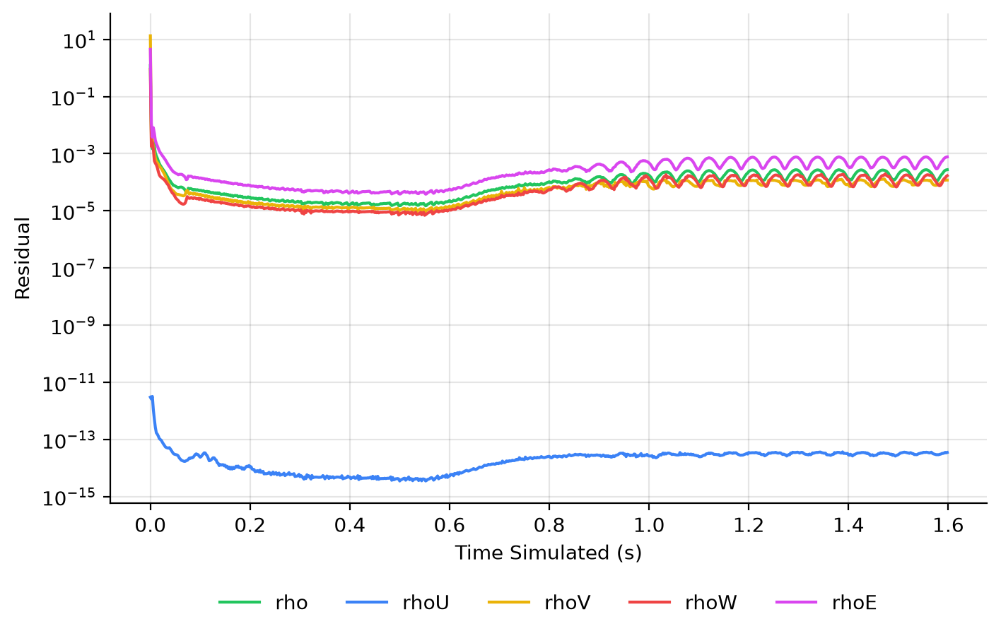
Each point is the residual at the end of a time step. They fall quickly from the uniform start, then sit between
10-5 and 10-3. Once shedding begins, from about 0.7 s, they rise a little and oscillate at the
shedding frequency: the flow is changing all the time, so there is no steady state for the residuals to fall
towards. `rhoV[0]`, the momentum along the span (x), stays near round-off throughout, because the flow has no
velocity in that direction.
### Monitor points
zMon's monitor points panel shows the `probe_cp` column the monitor adds to the report:
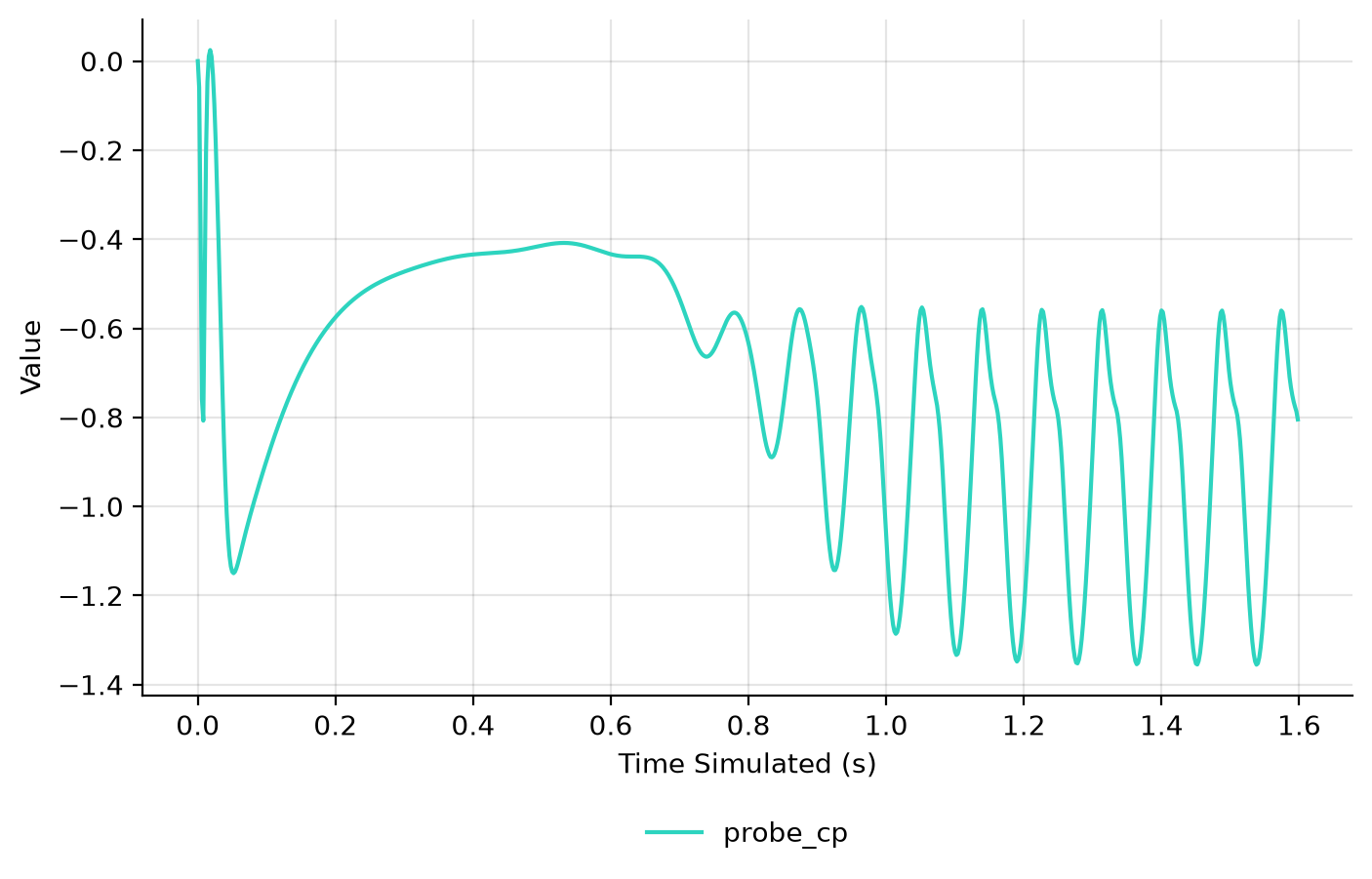
The pressure behind the cylinder settles at first, then from about 0.7 s starts to oscillate as the wake breaks
symmetry and vortices are shed. By 1.2 s the oscillation is regular. Its frequency gives the shedding frequency:
the cylinder sheds at 11.5 Hz. Engineers usually quote it as a Strouhal number, the frequency times the
diameter divided by the flow speed, which lets cylinders of any size and speed be compared: here it is 0.17.
## Step 5. Post-process
First activate your zCFD environment, which provides Python with zutil, h5py and ParaView:
```bash
source /bin/activate
```
### Python
This script draws the plots in [Step 4](#step-4-monitor) and measures the shedding frequency. It keeps the last report
row of each time step (`groupby("RealTimeStep").last()`) and turns the step number into time with the 0.002 s time
step. It then finds the peaks of `probe_cp` after 1.2 s, once the shedding is
regular: the frequency is the number of periods between the first and last peak divided by the time between them.
The Strouhal number divides by the flow speed, 66.82 m/s, which the log prints. Save the script as
`shedding_frequency.py` in the case directory:
```python
import matplotlib.pyplot as plt
from zutil.fileutils import get_zcfd_result
report = get_zcfd_result("cylinder.py").report.data
steps = report.groupby("RealTimeStep").last()
time = steps.index * 0.002
fig, ax = plt.subplots()
for column in ["rho", "rhoV[0]", "rhoV[1]", "rhoV[2]", "rhoE"]:
ax.semilogy(time, steps[column], label=column)
ax.set_xlabel("Time (s)")
ax.set_ylabel("Residual")
ax.legend()
fig.savefig("residuals.png", dpi=200)
fig, ax = plt.subplots()
ax.plot(time, steps["probe_cp"])
ax.set_xlabel("Time (s)")
ax.set_ylabel("probe_cp")
fig.savefig("probe.png", dpi=200)
cp = steps["probe_cp"].to_numpy()
peaks = [time[i] for i in range(1, len(cp) - 1) if time[i] > 1.2 and cp[i - 1] < cp[i] > cp[i + 1]]
frequency = (len(peaks) - 1) / (peaks[-1] - peaks[0])
print(f"Shedding frequency {frequency:.2f} Hz, Strouhal number {frequency * 1.0 / 66.82:.3f}")
```
Run it:
```bash
python shedding_frequency.py
```
It writes `residuals.png` and `probe.png`, and prints the shedding frequency and the Strouhal number:
```text
Shedding frequency 11.49 Hz, Strouhal number 0.172
```
### ParaView
#### Flow field
The solution output frequency is 5, so the solver writes visualisation data every 5 time steps. All of them are
stored in a single `cylinder.vtkhdf` file in the `cylinder_OUTPUT/cylinder/` directory.
Launch ParaView and load `cylinder_OUTPUT/cylinder/cylinder.vtkhdf`. ParaView shows one time step at a time, and
you can move through them with the icons at the top of the screen:

#### Animation
For unsteady data it is often useful to output an animation of the solution. This can be done in ParaView by
either exporting an image per timestep and then using a third party tool to stitch the images into a video or by
saving the animation directly. The advantage of the first approach is that it can easily be scripted and is more
suitable for large cases.
Since this case is small, this tutorial exports an mp4 video directly from ParaView. The steps to do this are:
1. Launch ParaView and load `cylinder_OUTPUT/cylinder/cylinder.vtkhdf`.
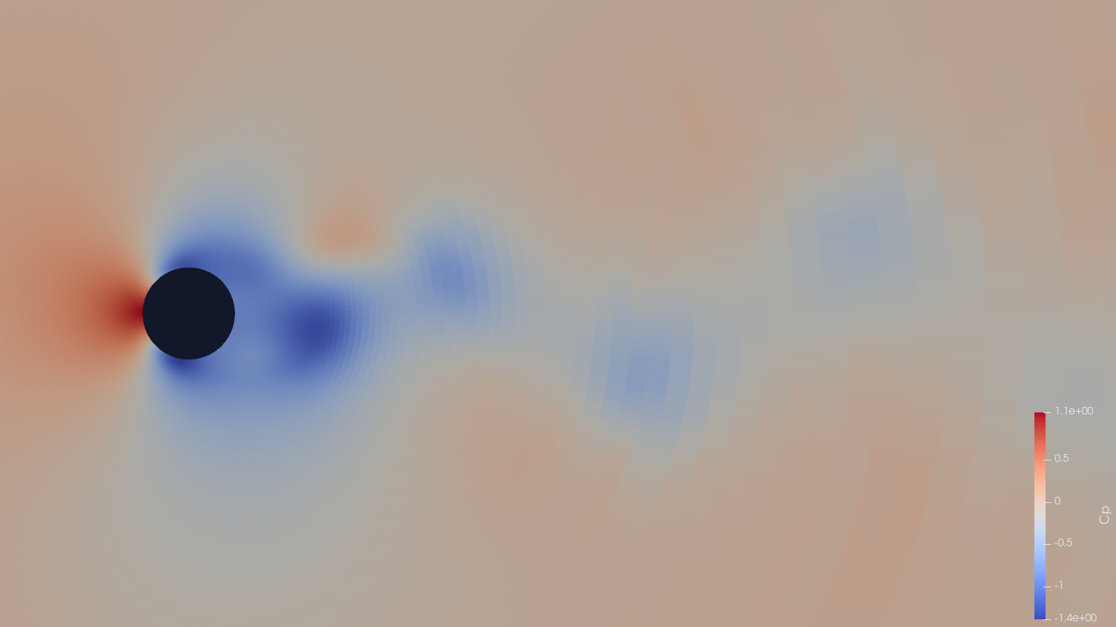
2. Set the view up to shade the output by _"cp"_ and zoom/move the image until you are happy with the view:
3. Select _'File->Save Animation'_ in ParaView. To export as video select your preferred format, the format will
depend on your Operating System but for Windows you should be able to select "MP4 files" and on Linux "FFMPEG
AVI". Give the file a name and click OK.
4. On the next screen you can set the target resolution, frame rate and the timesteps to export. Set the Image
resolution to 1920x1080 (FHD) and the frame rate to 24. To export only the end of the simulation (where the oscillation is established), set the Frame Window from 80 to 160.
5. Click OK to export the animation. This will take some time.
You should now have an exported video of the unsteady simulation.
:::