---
title: 5 · Overset meshes
section: tutorials
order: 50
---
# Overset meshes
## What is in this tutorial?
A CFD solver divides the space round an object into small cells, the _mesh_, and solves the flow equations in
each cell. An _overset_ mesh is a second mesh placed over the first. Where it lies, its cells take over: the cells
of the mesh beneath are switched off, which is called _hole cutting_. Along the edge of the overlap, the
_interface_, each mesh takes the values it needs from the nearest active cells of the other, its _donor_ cells.
This is useful when:
- a region needs a finer or different mesh than the one around it;
- a component is added to an existing mesh, such as a propeller on an aircraft, or a new building in a cityscape,
without regenerating the whole mesh;
- parts move relative to each other, such as a train entering a tunnel.
zCFD solves the flow separately on each mesh, finds where each mesh is active, and handles the exchange between all
of them, including when a run is split across several GPUs. Each overset boundary names the meshes it takes its data from.
[Overset meshes](../guide/working-with/overset-meshes.md) describes how this works.
This tutorial has two examples. The first places two cylinders over a refinement region over a background mesh, to
show how overset meshes are set up and viewed. The second moves a train into a tunnel and checks the pressure wave
it makes against a European standard.
## What you need?
Work through [Simple aerofoil](./1-simple-aerofoil.md) first. The cylinders take about two and a half minutes on an NVIDIA RTX 3060. The train
in a tunnel is far larger, about 8 million cells, and needs about 48 GB of GPU memory.
::: {.track when="deck"}
## Example 1. Overset cylinders
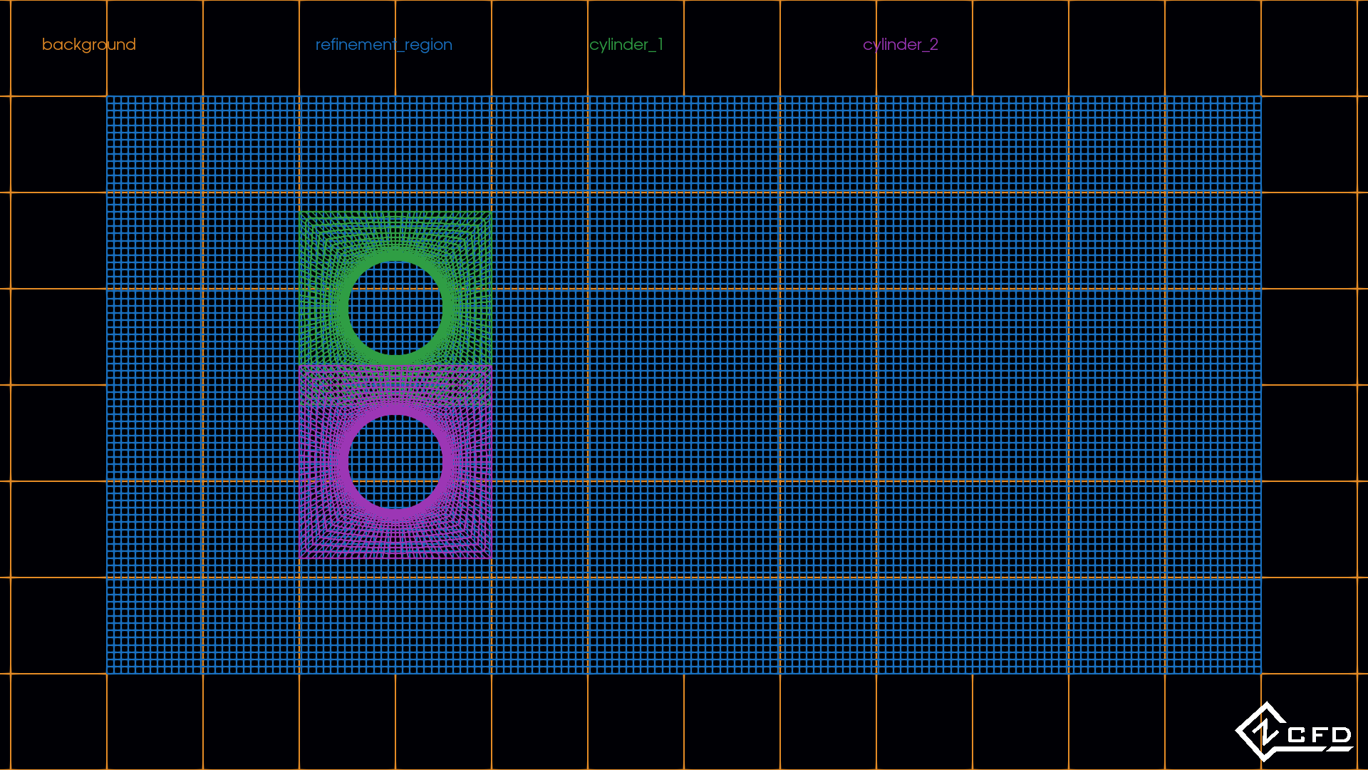
Four meshes make up this case: a coarse background, a finer refinement region over it, and a mesh round each of two
cylinders over that.
## Step 1. Download the files
The bundle can be downloaded [here](https://zcfd.zenotech.com/v2026.11.16174/tutorial_5_overset_cylinders.tgz).
```bash
cd ~
wget https://zcfd.zenotech.com/v2026.11.16174/tutorial_5_overset_cylinders.tgz
tar xzf tutorial_5_overset_cylinders.tgz
cd tutorial_5_overset_cylinders
```
It contains the control file `overset_cylinders.py` and three meshes: `background.h5`, `refinement_region.h5` and
`cylinder.h5`, which both cylinders use.
## Step 2. Walk through the input
The control file, `overset_cylinders.py`, is a short Python script. All it does is build one Python dictionary, called
`parameters`, that tells zCFD everything about the run: the physics, the numerical method, what to write out, and
the mesh with its boundaries. This step walks through that dictionary from top to bottom. Each heading below is the
name of a key, written exactly as it appears in the file, and the headings nest the same way the dictionary does:
`numerical scheme`, for example, sits inside `solver`. Under each heading you'll find what that part controls, what
each setting means, and why it has the value it has here. Each section ends with a link to that part's reference
page, which lists every setting it accepts and its default; you don't need it to follow the tutorial. On a wide
screen the whole control file sits on the right, with the part being described highlighted as you scroll.
Here `model` has one entry for each of the four meshes.
```python
parameters = {
"config version": 2,
"solver": {
"solver settings": {"type": "compressible"},
"equations": {"type": "viscous", "precondition": True},
"fluid properties": {
"material": "air",
"gamma": 1.4,
"gas constant": 287.0,
"sutherlands const": 110.4,
"prandtl no": 0.72,
"turbulent prandtl no": 0.9,
},
"reference conditions": {
"IC_1": {
"temperature": 277.7777,
"pressure": 101325.0,
"v": {"vector": [1.0, 0.0, 0.0], "mach": 0.2},
"reynolds no": 20.0,
"reference length": 1.0,
}
},
"initialisation": {"initial conditions": "IC_1"},
"numerical scheme": {"order": "second"},
"time settings": {"type": "steady"},
"convergence control": {
"scheme": {"name": "implicit euler", "stage": 1},
"cfl": {
"cfl": 20,
"cfl viscous factor": 1.0e-6,
"cfl ramp": [{"type": "exponential", "factor": 1.05, "initial": 0.1}],
},
"cycles": 2000,
},
"output settings": {
"report": {
"frequency": 5,
"monitor": {
"MR_1": {
"name": "probe",
"point": [1.07, 0.25, 0.313],
"variables": ["cp"],
}
},
},
"solution": {
"format": "vtk",
"surface variables": ["V", "p", "T", "rho", "cp"],
"volume variables": ["V", "p", "T", "rho", "mach", "cp", "overset"],
},
},
},
"model": {
"background": {
"mesh": "background.h5",
"transforms": {
"transform": [
[1.0, 0.0, 0.0, 0.0],
[0.0, 1.0, 0.0, 0.0],
[0.0, 0.0, 1.0, -0.5],
[0.0, 0.0, 0.0, 1.0],
]
},
"boundary conditions": {
"BC_1": {"zones": [9, 11], "type": "symmetry"},
"BC_2": {
"zones": [10],
"type": "farfield",
"condition": "IC_1",
"kind": "riemann",
},
},
},
"refinement_region": {
"mesh": "refinement_region.h5",
"boundary conditions": {
"BC_1": {"zones": [9, 11], "type": "symmetry"},
"BC_2": {
"zones": [10],
"type": "interface",
"kind": "overset",
"connection": {"model": ["background"]},
"additional active layers": 3,
},
},
},
"cylinder_2": {
"mesh": "cylinder.h5",
"transforms": {
"transform": [
[1.0, 0.0, 0.0, 0.0],
[0.0, 1.0, 0.0, -0.8],
[0.0, 0.0, 1.0, 0.0],
[0.0, 0.0, 0.0, 1.0],
]
},
"boundary conditions": {
"BC_1": {"zones": [11, 12], "type": "symmetry"},
"BC_2": {
"zones": [13],
"type": "interface",
"kind": "overset",
"connection": {"model": ["refinement_region"]},
"additional active layers": 3,
},
"BC_3": {"zones": [10], "type": "wall", "kind": "no slip"},
},
},
"cylinder_1": {
"mesh": "cylinder.h5",
"transforms": {
"transform": [
[1.0, 0.0, 0.0, 0.0],
[0.0, 1.0, 0.0, 0.8],
[0.0, 0.0, 1.0, 0.0],
[0.0, 0.0, 0.0, 1.0],
]
},
"boundary conditions": {
"BC_1": {"zones": [11, 12], "type": "symmetry"},
"BC_2": {
"zones": [13],
"type": "interface",
"kind": "overset",
"connection": {"model": ["refinement_region"]},
"additional active layers": 3,
},
"BC_3": {"zones": [10], "type": "wall", "kind": "no slip"},
},
},
},
}
```
### `config version`
`"config version": 2` says which layout of the control file this is. It may be written with a space or an underscore.
### `solver`
`solver` holds the settings shared by all four meshes.
#### `solver settings`
[`solver settings`](/reference/solver/solver-settings) chooses the solver.
- `type`: `compressible`, the density-based solver.
#### `equations`
[`equations`](/reference/solver/equations) sets which equations are solved.
- `type`: `viscous`, the laminar Navier–Stokes equations; the flow round each cylinder is laminar at a Reynolds
number of 20. The Reynolds number compares the flow's inertia with its viscosity.
- `precondition`: `True`, low-Mach-number preconditioning, recommended below about Mach 0.3.
#### `fluid properties`
[`fluid properties`](/reference/solver/fluid-properties) describes the gas.
- `material`: `air`, an ideal gas, with `gamma` 1.4 and `gas constant` 287.0 J/kg/K.
- `sutherlands const`: 110.4 K, for the viscosity's change with temperature.
- `prandtl no` 0.72 and `turbulent prandtl no` 0.9; the turbulent one plays no part in a laminar run.
#### `reference conditions`
[`reference conditions`](/reference/solver/reference-conditions) defines named flow states.
##### `IC_1`
`IC_1` is the freestream.
- `temperature` 277.7777 K and `pressure` 101325 Pa.
- `v`: `vector` [1, 0, 0] and `mach` 0.2, so the flow runs along +x at 66.8 m/s.
- `reynolds no`: 20, based on the `reference length`, 1.0 m, the diameter of each cylinder. Above a Reynolds
number of about 47, a single cylinder sheds vortices: they peel off alternately behind it, so the flow never
settles to a steady state. Two cylinders 1.6 diameters apart behave more like one
wider body, so they start to shed sooner; 20 is chosen to stay below that, so the flow settles to a steady state.
The run confirms it by converging.
#### `initialisation`
[`initialisation`](/reference/solver/initialisation) sets the starting state.
- `initial conditions`: `IC_1` in every cell of every mesh.
#### `numerical scheme`
[`numerical scheme`](/reference/solver/numerical-scheme) sets the spatial discretisation.
- `order`: `second`, with the default Roe flux and van Albada limiter.
[Choosing a limiter](../guide/choosing/choosing-a-limiter.md) covers both.
#### `time settings`
[`time settings`](/reference/solver/time-settings) says how the run advances.
- `type`: `steady`. The flow at this Reynolds number does not change in time, so the solver simply iterates, in a
made-up _pseudo-time_, until the solution stops changing. [Choosing a time-marching scheme](../guide/choosing/choosing-a-time-marching-scheme.md)
explains the choice.
#### `convergence control`
[`convergence control`](/reference/solver/convergence-control) sets how the pseudo-time iterations converge to the
steady state.
##### `scheme`
- `name`: `implicit euler`. An overset case needs an implicit pseudo-time scheme; see
[Practical consequences](../guide/working-with/overset-meshes.md#practical-consequences).
- `stage`: 1. It has no effect under implicit Euler, which has only one stage.
##### `cfl`
- `cfl`: 20, the pseudo-time CFL number. This overset stack diverges in its first cycles at 100 or more.
- `cfl viscous factor`: 1.0e-6. It scales the viscous part of each cell's pseudo-time step estimate, so at this
value the convective wave speeds alone set the step.
- `cfl ramp`: starts at 0.1 and grows by 1.05 a cycle, so the first cycles, from a flow that has not yet seen the
cylinders, are gentle.
##### `cycles`
- `cycles`: 2000, enough for the residuals, which measure how far the equations are from being satisfied, to fall
several orders of magnitude, and for the probe to settle.
#### `output settings`
[`output settings`](/reference/solver/output-settings) sets the report, written as the run goes, and the solution
files. Each model gets its own report and solution files, in its own folder.
##### `report`
- `frequency`: a row every 5 cycles in each model's report, with that model's residuals.
- `monitor`: `MR_1`, `name`d `probe`, records `cp` at the `point` [1.07, 0.25, 0.313], between and behind the
cylinders. Every model's report has the column `probe_cp`, but only the model whose active cell holds the point
fills it: here the refinement region. In the others it stays zero.
##### `solution`
- `format`: `vtk`, VTK HDF files for ParaView.
- `surface variables`: `V`, `p`, `T`, `rho` and `cp` on each model's boundaries.
- `volume variables`: the same, with `mach`, and `overset`: 0 in a cell another mesh has taken over, 1 in a cell
that is active, and 2 in a cell kept active only by `additional active layers`, in the band where two meshes
overlap. [Step 5](#step-5-post-process) uses it to show only the active cells.
- With no `frequency` set, the solution files and the checkpoint are written once, at the end of the run.
### `model`
[`model`](/reference/model) has one entry for each mesh. Each name, such as `background`, names that model's output
folder, `overset_cylinders_OUTPUT/background/`, and its files. The order matters: each mesh oversets meshes before
it in the list. `background` is walked in full below; the others differ only as each says.
#### `background`
The coarse mesh beneath the others, 100 m square.
##### `mesh`
`background.h5`, 10,000 cells.
##### `transforms`
[`transforms`](/reference/model/transforms) places the mesh when it is read.
- `transform`: a 4 × 4 matrix whose last column translates the mesh. Here it moves the mesh 0.5 m down z, so that its
span, built from z = 0.5 to 1.5, lines up with the other meshes' span, z = 0 to 1.
[Placing and moving a mesh](../guide/working-with/placing-and-moving-a-mesh.md) describes the matrix.
##### `boundary conditions`
[`boundary conditions`](/reference/model/boundary-conditions) assign a condition to each group of the mesh's zones.
###### `BC_1`
- `zones` [9, 11], the two faces normal to the span, `type` `symmetry`, so one cell across the span is enough.
###### `BC_2`
- `zones` [10], the outer boundary, `type` [`farfield`](../guide/choosing/choosing-boundary-conditions.md#farfield)
with `condition` `IC_1` and `kind` `riemann`.
#### `refinement_region`
A finer Cartesian mesh round both cylinders, 12,800 cells in `refinement_region.h5`, with no transform.
##### `boundary conditions`
Its `BC_1` is the same symmetry. Its `BC_2` is where it meets the background:
###### `BC_2`
- `zones`: [10], the outer boundary of the refinement region.
- `type` `interface` and `kind` `overset`: the boundary of an overset mesh. The background cells that lie under
the refinement region are not solved, and the two meshes exchange the solution across this boundary.
- `connection`: `model` `["background"]`, the mesh it takes its data from. Naming it tells the solver exactly which
pair of meshes to map; without it, the solver maps against every model before this one.
- `additional active layers`: 3. The hole the refinement region cuts in the background would otherwise match its
own outline exactly, leaving no band where both meshes are solved, and the interface faces would find no active
cell to take their data from. Three extra layers of background cells are kept active round the hole, so the two
meshes overlap. [Donor search](../guide/working-with/overset-meshes.md#donor-search) explains why this matters.
[Overset interface](../guide/working-with/overset-meshes.md#overset-interface) lists its other settings.
#### `cylinder_2`
The lower cylinder: `cylinder.h5`, 5040 cells round a cylinder of 1 m diameter.
- `transforms`: `transform` moves it 0.8 m down y.
- `BC_1`: symmetry on zones [11, 12].
- `BC_2`: an overset interface on zone 13, its outer boundary, with `connection` `model` `["refinement_region"]` and,
for the same reason as the refinement region's, `additional active layers` 3.
- `BC_3`: zone 10, the cylinder surface, a no-slip `wall`.
#### `cylinder_1`
The upper cylinder: the same mesh and conditions as `cylinder_2`, moved 0.8 m up y instead. One mesh file can serve
several models, each placed by its own transform.
The two cylinder meshes overlap each other between the cylinders. That is allowed, because each names its own
donor, the refinement region; in each place the solution is taken from the topmost mesh.
## Step 3. Run
In the activated environment, check the control file and run it:
```bash
cd ~/tutorial_5_overset_cylinders/
validate_input overset_cylinders.py
run_zcfd -c overset_cylinders.py
```
All four meshes are read from the `mesh` key of each model. These are extracts from the log of a run of this
tutorial, `overset_cylinders.log`, with `...` marking lines left out:
```text
Parameters validated successfully
...
Reading file background.h5
Global Mesh Stats: Cells: 10000 Faces: 40200
...
Reading file refinement_region.h5
Global Mesh Stats: Cells: 12800 Faces: 51440
...
Reading file cylinder.h5
Global Mesh Stats: Cells: 5040 Faces: 20280
...
Overset hole cut: blanked 168 background cells enclosed by the hole (inside the overset mesh's solid bodies)
...
Overset mapping: 104 of 288 (36.1111%) background halo centres found no active donor cell in the overset mesh. Those faces fall back to the unmapped face treatment instead of interpolated data. The meshes do not overlap deeply enough: increase 'additional active layers' on the overset interface.
...
============================================================
Overset Mesh Hierarchy (4 models, 6 pairs)
============================================================
background [root]
└── refinement_region [overset]
├── cylinder_2 [overset]
└── cylinder_1 [overset]
Peer overlaps: background ↔ cylinder_2, background ↔ cylinder_1, cylinder_2 ↔ cylinder_1
============================================================
...
Solve Complete: 2000 cycles in 2m 27.7s (avg 73.8 ms/cycle)
...
zCFD finished: all requested cycles are complete (2000 in total).
```
- Each mesh is read in turn; `cylinder.h5` is read twice, once for each cylinder.
- The hole cut blanks the background cells inside each cylinder.
- The hierarchy shows which mesh oversets which, as the `connection` entries ask.
- As the run goes, a report box every few cycles gives each model's residuals separately.
- The log may print a few lines starting `Overset mapping:`. Each reports the share of an interface's halo cells,
the extra cells along the interface that hold the other mesh's values, that found no active donor cell to take
data from; those faces use the unmapped-face treatment
instead of interpolated data. They are diagnostics, not errors. The three `additional active layers` set above
reduce them, and this case converges cleanly with the few that remain.
[Donor search](../guide/working-with/overset-meshes.md#donor-search) explains these lines.
- The run ends after its 2000 cycles.
### Output files
| File/Directory | Description |
| --------------------------------------------- | -------------------------------------------------------------- |
| `overset_cylinders.log` | A copy of the output to screen during the run. |
| `overset_cylinders_status.yaml` | How the run was started: version, date, control file, meshes. |
| `overset_cylinders_OUTPUT/background/` | The background's report, checkpoint, volume and surface files. |
| `overset_cylinders_OUTPUT/refinement_region/` | The same for the refinement region. |
| `overset_cylinders_OUTPUT/cylinder_1/` | The same for the upper cylinder. |
| `overset_cylinders_OUTPUT/cylinder_2/` | The same for the lower cylinder. |
| `overset_cylinders_OUTPUT/LOGGING/` | A separate log for each MPI rank, used for debugging. |
Each model folder holds files named after the model, such as `cylinder_1/cylinder_1_report.csv` and
`cylinder_1/cylinder_1.vtkhdf`.
## Step 4. Monitor
Open the run in zMon:
```bash
zmon overset_cylinders.py
```
zMon shows each model's residuals and monitors against cycle;
[Monitoring a run](../guide/working-with/monitoring-a-run.md) describes the panels.
- Each model has its own residuals. The cylinder meshes start with the largest, as the flow first meets the
cylinders, and fall more than four orders of magnitude. The refinement region starts from the uniform freestream,
so its residual starts near zero, rises as the disturbance reaches it, then falls. The background's residual stays
at round-off level, around 10-18, throughout.
- The `probe_cp` monitor sits in the wake between and behind the cylinders. Choose the refinement region's report:
it is the mesh whose active cell holds the point, and the other models show zero. Once the run has converged the
probe holds a steady value.
## Step 5. Post-process
First activate your zCFD environment, which provides Python with zutil, h5py and ParaView:
```bash
source /bin/activate
```
### Python
This script prints each model's largest and final density residual, and the final value at the probe. Save it as
`print_convergence.py` beside the control file:
```python
from zutil.fileutils import get_zcfd_result
result = get_zcfd_result("overset_cylinders.py")
for model, report in result.model_reports.items():
rho = report.data["rho"]
print(f"{model}: density residual fell from {rho.max():.1e} to {rho.iloc[-1]:.1e}")
probe = result.model_reports["refinement_region"].data["probe_cp"]
print(f"probe cp at the end of the run: {probe.iloc[-1]:.3f}")
```
```bash
python print_convergence.py
```
### ParaView
Overset meshes keep their solutions separate, so you can load only the meshes covering the region you want. To
view the whole domain as one, combine them in ParaView:
- Load the four files `overset_cylinders_OUTPUT/background/background.vtkhdf`,
`.../refinement_region/refinement_region.vtkhdf`, `.../cylinder_1/cylinder_1.vtkhdf` and
`.../cylinder_2/cylinder_2.vtkhdf`.
::: {.note}
To make this easier, `generate_paraview_helpers` writes ParaView scripts that load every model's output for you.
Run it, then run the volume script once with `pvpython` to save its state:
```bash
(zCFD)> generate_paraview_helpers overset_cylinders.py
(zCFD)> pvpython paraview_view_volumes.py
```
Open `paraview_view_volumes.pvsm` with _File > Load State…_ to load all four volumes, each in its own colour. The
overset cells are still there; the steps below remove them. See
[Opening a run in ParaView](../guide/working-with/post-processing-and-visualisation.md#opening-a-run-in-paraview).
:::
- Select all four in the pipeline browser and apply _Filters > Group Datasets_. The new _GroupDatasets1_ holds all
four.
- Apply _Filters > Merge Blocks_ to _GroupDatasets1_. ParaView reads each .vtkhdf file as one block per partition,
which _Append Datasets_ cannot take; _MergeBlocks1_ is a single dataset holding the cells of all four meshes.
- Apply _Filters > Threshold_ to _MergeBlocks1_ on the `overset` variable, with the lower threshold raised from 0
to 1. _Threshold1_ keeps only the active cells.
- Apply _Filters > Cell Data to Point Data_ to _Threshold1_, which makes later interpolation more accurate.
- Apply _Filters > Slice_ with its normal along z. The slice holds data from all four meshes.
- Colour _Slice1_ by `V` _Magnitude_, with _Surface With Edges_ in the representation toolbar.
Streamlines and other filters work the same way. Where meshes move during an unsteady run, ParaView updates their
positions.
The cylinder meshes have holes where the cylinders are, so the refinement region shows through behind them. To hide
it, add a cylinder of unit diameter with _Sources > Cylinder_ at [0, 0, 0], rotate it 90° about x and translate it
by −0.8 in y; repeat with +0.8 for the other cylinder. The view then looks like this:
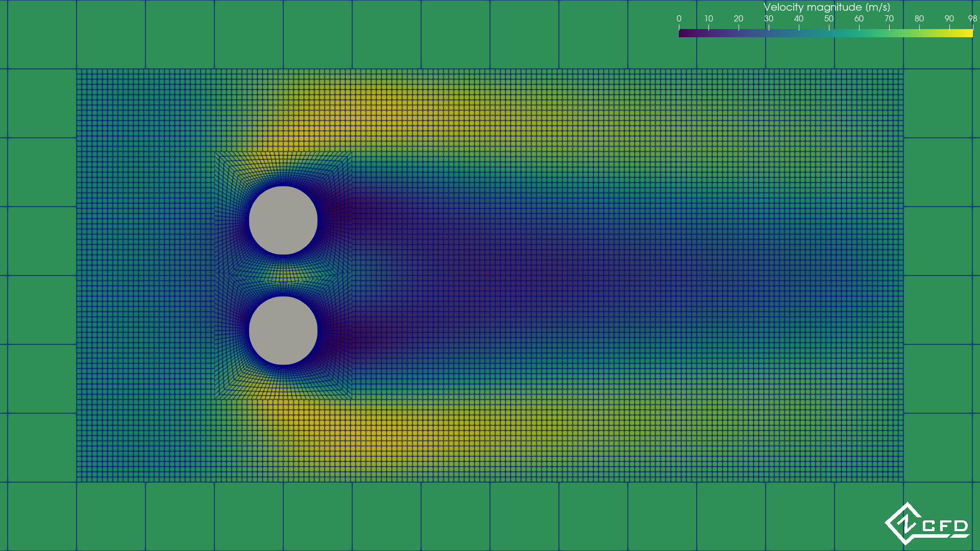
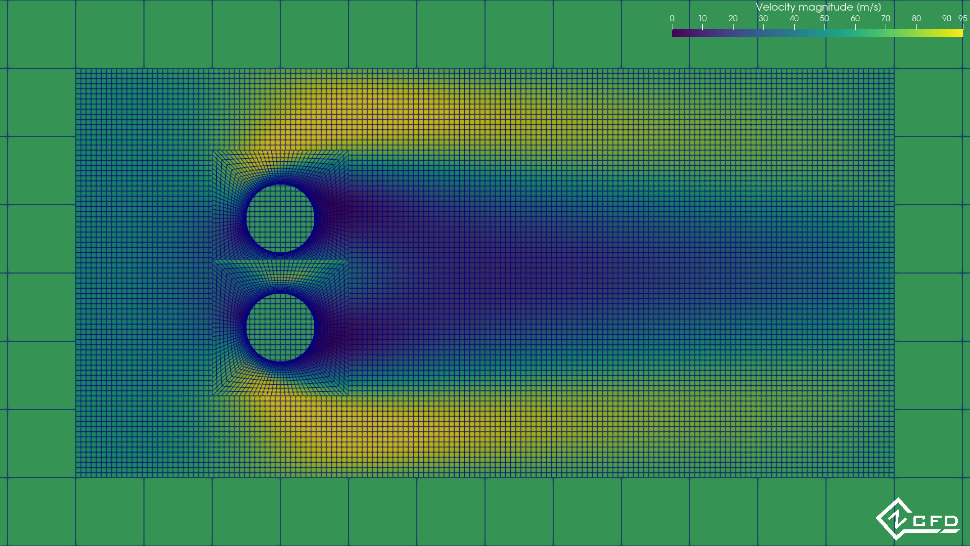
To bring the cylinder meshes to the front instead, view each mesh separately and give each cylinder mesh a small
offset towards the viewer, normal to the slice (0.0, 0.001, 0.0015, 0.002). That is closer to what the solver
sees, since the covered cells of the meshes beneath are not solved.
## Example 2. Train in a tunnel
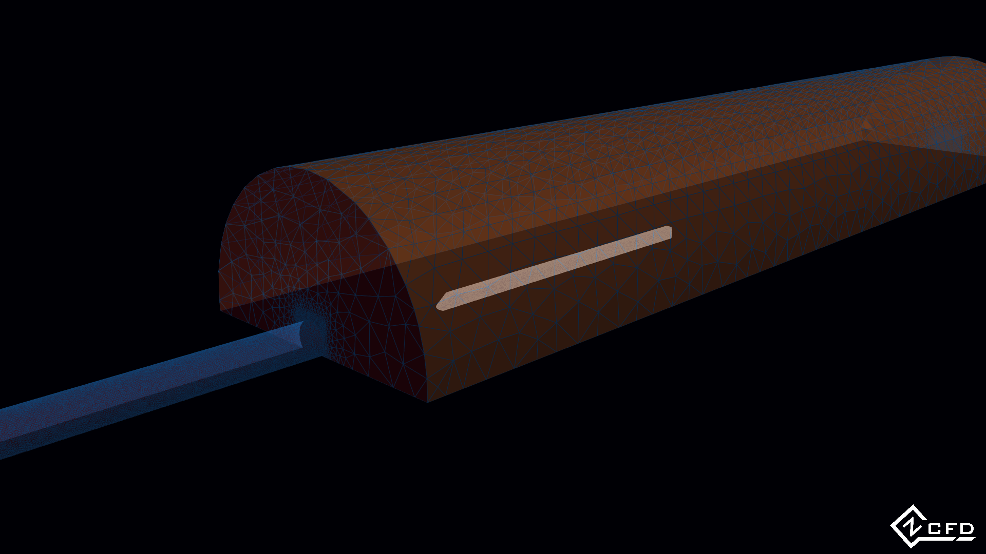
A train entering a tunnel pushes a pressure wave ahead of it, which leaves the far end as a micro pressure wave: a
boom. This example predicts the wave, with the set-up of Section 7.6 of EN 14067-5, _Railway applications —
Aerodynamics — Part 5: Requirements and test procedures for aerodynamics in tunnels_ [[1]](#citations). For the
reference train entering the reference tunnel at 250 km/h, the maximum entry pressure gradient dp/dt should lie
between 8800 Pa/s and 9700 Pa/s.
## Step 1. Download the files
The bundle can be downloaded [here](https://zcfd.zenotech.com/v2026.11.16174/traintunnel.tgz).
```bash
cd ~
wget https://zcfd.zenotech.com/v2026.11.16174/traintunnel.tgz
tar xzf traintunnel.tgz
cd traintunnel
```
It contains the control file `traintunnel.py` and two meshes: `tunnel.h5`, 7.07 million cells, and `train.h5`,
1.06 million.
## Step 2. Walk through the input
The control file, `traintunnel.py`, is a short Python script. All it does is build one Python dictionary, called
`parameters`, that tells zCFD everything about the run: the physics, the numerical method, what to write out, and
the mesh with its boundaries. This step walks through that dictionary from top to bottom. Each heading below is the
name of a key, written exactly as it appears in the file, and the headings nest the same way the dictionary does:
`numerical scheme`, for example, sits inside `solver`. Under each heading you'll find what that part controls, what
each setting means, and why it has the value it has here. Each section ends with a link to that part's reference
page, which lists every setting it accepts and its default; you don't need it to follow the tutorial. On a wide
screen the whole control file sits on the right, with the part being described highlighted as you scroll.
Here `model` has two entries, the tunnel and the train. Where a block works as in the cylinders above, it
is covered briefly.
```python
parameters = {
"config version": 2,
"solver": {
"solver settings": {"type": "compressible"},
"initialisation": {"initial conditions": "IC_1"},
"equations": {"type": "euler"},
"reference conditions": {
"IC_1": {
"temperature": 292.7777,
"pressure": 101325.0,
"v": {"vector": [1.0, 0.0, 0.0], "mach": 1e-10},
"reference length": 1.0,
}
},
"time settings": {
"type": "unsteady",
"kind": "dual time stepping",
"total time": 3.6,
"time step": 0.001,
"start": 0,
"order": 1,
},
"convergence control": {
"scheme": {"name": "implicit euler", "stage": 1},
"cfl": {"cfl": 30},
"cycles": 5,
},
"numerical scheme": {
"order": "second",
},
"fluid properties": {
"material": "ideal gas",
"gamma": 1.4,
"gas constant": 287.0,
"sutherlands const": 110.4,
"prandtl no": 0.72,
},
"output settings": {
"report": {
"frequency": 10,
"monitor": {
"MR_1": {
"name": "probe",
"point": [-140, 1.5, 0],
"variables": ["p"],
}
},
},
"solution": {
"format": "vtk",
"surface variables": ["overset", "V", "p", "T", "rho"],
"volume variables": ["overset", "V", "p", "T", "rho", "m", "sponge"],
},
},
},
"model": {
"background": {
"mesh": "tunnel.h5",
"boundary conditions": {
"BC_1": {"zones": [11, 13], "type": "symmetry"},
"BC_2": {
"zones": [12],
"type": "farfield",
"kind": "riemann",
"condition": "IC_1",
"sponge layer damping": {
"distance": 20.0,
"damping factor": 2.037495,
"condition": "IC_1",
},
},
},
},
"train": {
"mesh": "train.h5",
"transforms": {
"transform": [
[1.0, 0.0, 0.0, 110.0],
[0.0, 1.0, 0.0, 0.0],
[0.0, 0.0, 1.0, 0.0],
[0.0, 0.0, 0.0, 1.0],
],
"motion": {
"type": "translating",
"velocity": [-69.4, 0.0, 0.0],
"moving mesh": True,
"ramp time": 1.5,
},
},
"boundary conditions": {
"BC_1": {"zones": [10], "type": "symmetry"},
"BC_2": {
"zones": [9],
"type": "interface",
"kind": "overset",
"create overset halos": False,
"interpolation method": "nearest cell",
},
"BC_3": {"zones": [8], "type": "wall", "kind": "slip"},
},
},
},
}
```
### `config version`
`"config version": 2`, the layout of the control file.
### `solver`
`solver` holds the settings shared by both meshes.
#### `solver settings`
- `type`: `compressible`, the density-based solver.
#### `initialisation`
- `initial conditions`: `IC_1` in every cell: still air everywhere, with the train at rest.
#### `equations`
- `type`: `euler`, the inviscid Euler equations. The pressure wave is a compressible, inviscid effect, so viscosity
is left out, which keeps a case of this size affordable.
#### `reference conditions`
##### `IC_1`
- `temperature` 292.7777 K (19.6 °C) and `pressure` 101325 Pa.
- `v`: `vector` [1, 0, 0] and `mach` 1e-10: still air. The train moves; the air does not. The Mach number is not set
to exactly zero, because the solver scales by it.
- `reference length`: 1.0 m.
#### `time settings`
- `type` `unsteady`, `kind` `dual time stepping`: the train moves, so the run follows the flow in time. Each
physical time step is solved like a small steady problem, by the inner iterations set in `convergence control`.
- `total time`: 3.6 s, long enough for the train to accelerate and enter the tunnel.
- `time step`: 0.001 s, 3600 steps.
- `start`: 0, no steady cycles first.
- `order`: 1, first order in time.
#### `convergence control`
- `scheme`: `implicit euler`. Its `stage` of 1 has no effect.
- `cfl`: 30, without a ramp.
- `cycles`: 5 inner cycles per time step.
#### `numerical scheme`
- `order`: `second`, with the default Roe flux and van Albada limiter.
#### `fluid properties`
- `material`: `ideal gas`, with `gamma` 1.4 and `gas constant` 287.0 J/kg/K.
- `sutherlands const` and `prandtl no` play no part in an Euler run, which has no viscosity or heat conduction.
#### `output settings`
##### `report`
- `frequency`: a row every 10 cycles.
- `monitor`: `MR_1`, `name`d `probe`, records the pressure `p` at the `point` [-140, 1.5, 0], inside the tunnel. It
falls in the tunnel mesh, so its column `probe_p` is filled in
`traintunnel_OUTPUT/background/background_report.csv`. Its history gives the entry pressure gradient in Step 5.
##### `solution`
- `format`: `vtk`, VTK HDF files for ParaView.
- `surface variables`: `overset`, `V`, `p`, `T` and `rho`.
- `volume variables`: the same, with the Mach number `m` and `sponge`, the damping applied by the sponge layer
below.
### `model`
#### `background`
The tunnel and the air round it. Its name gives the output folder, `traintunnel_OUTPUT/background/`.
##### `mesh`
`tunnel.h5`, 7.07 million cells.
##### `boundary conditions`
###### `BC_1`
- `zones` [11, 13], `type` `symmetry`.
###### `BC_2`
- `zones`: [12], the outer boundary.
- `type`: `farfield`, with `kind` `riemann` and `condition` `IC_1`.
- `sponge layer damping`: within `distance` 20 m of the farfield, the solution is damped towards its `condition`,
`IC_1`, at a rate rising to the `damping factor`, 2.037495, at the boundary. The sponge absorbs pressure waves
before they reach the farfield, where they would reflect back into the domain.
#### `train`
The train, with its output in `traintunnel_OUTPUT/train/`.
##### `mesh`
`train.h5`, 1.06 million cells.
##### `transforms`
- `transform`: a 4 × 4 matrix whose last column places the train 110 m along x before it starts to move.
- `motion`: how the train moves during the run.
- `type`: `translating`, a straight-line motion.
- `velocity`: [-69.4, 0, 0] m/s, 250 km/h towards −x and the tunnel.
- `moving mesh`: `True`, so the train mesh itself moves through the tunnel mesh. Every time step it is moved to
the position the motion gives at the end of the step, and its overset mappings are recalculated.
- `ramp time`: 1.5 s. The speed rises linearly from rest to the full velocity over the first 1.5 s, which avoids
the transients of an impulsive start.
A moving mesh is allowed only in an unsteady compressible run, on a mesh that also has an overset or sliding
interface. [Placing and moving a mesh](../guide/working-with/placing-and-moving-a-mesh.md) describes `transforms`.
##### `boundary conditions`
###### `BC_1`
- `zones` [10], `type` `symmetry`.
###### `BC_2`
- `zones` [9], the outer boundary of the train mesh, `type` `interface`, `kind` `overset`. It names no
`connection`, so it is mapped against every model before it: here only the tunnel.
- `create overset halos`: `False`. Donor values are taken at the boundary face centres. The default samples
at the halo cell centres, just outside the train mesh. On this moving train, some of those points have no donor
in the tunnel mesh.
- `interpolation method`: `nearest cell`: each point takes the value of the donor cell that contains it.
###### `BC_3`
- `zones`: [8], the train's surface.
- `type` `wall` with `kind` `slip`: in the Euler equations the flow slides along a wall rather than stopping at it.
## Step 3. Run
The case needs about 48 GB of GPU memory. Run it in the activated environment:
```bash
validate_input traintunnel.py
run_zcfd -c traintunnel.py
```
## Step 4. Monitor
```bash
zmon traintunnel.py
```
zMon shows each model's residuals, and the `probe_p` monitor in the reports panel of the background model: the
pressure inside the tunnel rising as the train enters.
## Step 5. Post-process
First activate your zCFD environment, which provides Python with zutil, h5py and ParaView:
```bash
source /bin/activate
```
### Python
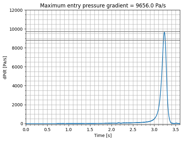
This script plots the entry pressure gradient: how fast the pressure inside the tunnel rises, the time derivative
of `probe_p`. Save it as `plot_entry_pressure_gradient.py` in the case directory:
```python
import matplotlib.pyplot as plt
import numpy as np
from zutil.fileutils import get_zcfd_result
time_step = 0.001
result = get_zcfd_result("traintunnel.py")
p = np.array(result.model_reports["background"].get_array("probe_p"))
dpdt = np.diff(p) / time_step
time = time_step * np.arange(len(dpdt))
fig, ax = plt.subplots()
ax.minorticks_on()
ax.grid(which="both")
ax.set_title(f"Maximum entry pressure gradient = {dpdt.max():.1f} Pa/s")
ax.set_xlabel("Time [s]")
ax.set_ylabel("dPdt [Pa/s]")
ax.set_xlim(0, 3.6)
ax.set_ylim(-100, 12000)
ax.plot(time, dpdt, label="250 km/h")
ax.axhline(8800, label="min valid dP/dT", c="grey")
ax.axhline(9700, label="max valid dP/dT", c="grey")
ax.legend()
fig.savefig("EntryPressureGradient.png")
```
Run it:
```bash
python plot_entry_pressure_gradient.py
```
It plots the entry pressure gradient against time. The maximum is 9660 Pa/s, within the 8800 Pa/s to 9700 Pa/s
the standard specifies.
:::
## Citations
1. EN 14067-5:2006 - Railway applications - Aerodynamics - Part 5: Requirements and test procedures for
aerodynamics in tunnels, [see](https://standards.iteh.ai/catalog/standards/cen/ea6cb49e-c40a-4b8b-a059-c6debdb91dc7/en-14067-5-2006)