Troubleshooting
CFD solvers can sometimes fail to converge or even crash when running. zCFD includes an automatic validation to ensure that the inputs are consistent and syntactically correct, and there are some common problems that can be identified even if the code has crashed.
Crashing
There are several common causes of code crashing:
Numerical instability
Inconsistent boundary conditions
Preconditioning
Poor mesh quality
Numerical instability
The solver will try to advance the flow solution towards convergence at the required level of spatial and temporal accuracy, subject to a user-defined limit called the CFL (Courant–Friedrichs–Lewy) number. The CFL number limits the update to the solution in each cycle to maintain the stability of the underlying numerical scheme.
There are formal criteria for the CFL number for given schemes, however these typically only apply to idealised (orthogonal or structured meshes with very gradual variation in cell-to-cell volume ratios). For complex meshes or where cell quality may be poor (even in only a few cells), the limit for stability may be significantly less. In explicit mode, the theoretical CFL limit is formally approximately 1.0 for most schemes - though in many cases a higher value (1.5 to 2.0) will actually work. In implicit mode the CFL limit is theoretically 1000 or more, with values between 10 and 100 quite common.
The solver will provide some feedback as it is running that can be helpful in diagnosing stability issues.
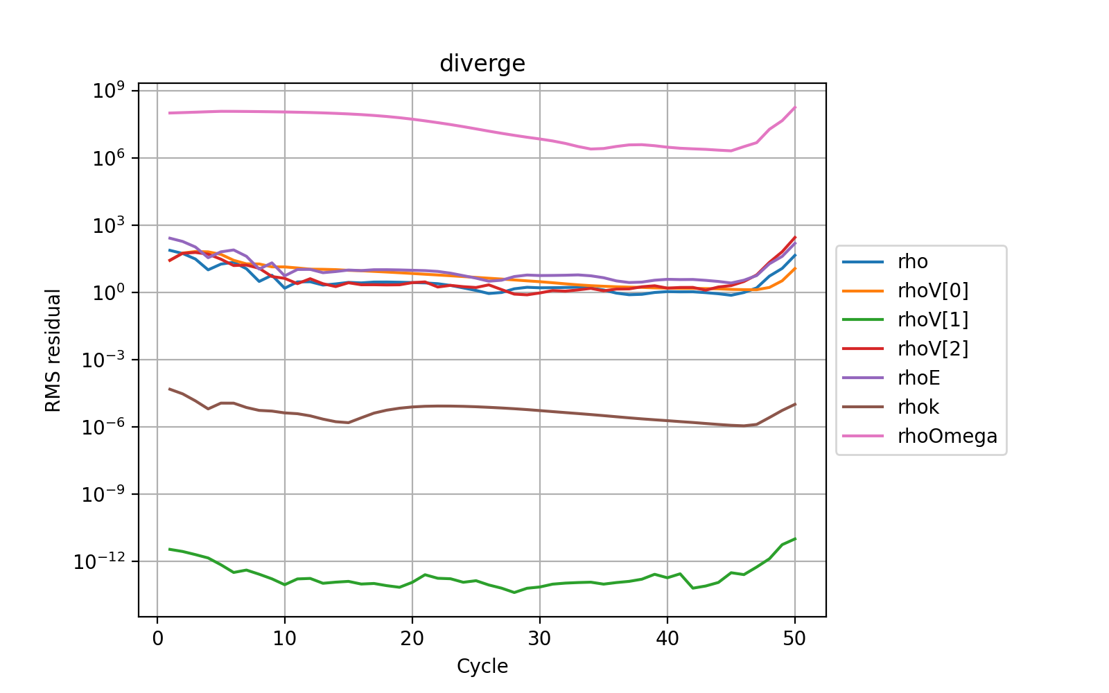
Fig. 6 The typical form of a divergent set of residuals. Rather than decreasing, the values all start increasing significantly from cycle 45 onwards. In this case the NACA0012 case was deliberately set with an unstable explicit CFL number of 6.0.
The residuals that are output in the _report.csv file should gradually reduce as the solver converges (per real time step if the flow is unsteady). If one or more of the reported values starts diverging, there is a good chance that the scheme has become unsteady. Note that this can also be a consequence of a particular pattern in the flow that appears during the solution process and so this divergence may occur after a period of otherwise stable convergence. For implicit runs using the AMGX library, reporting includes the number of cycles of the implicit linear solver and the residual value associated with each. Typically 4 to 5 cycles should be enough. If the number of iterations to achieve the desired improvement in accuracy (typically 3 to 4 orders of magnitude) starts increasing above 6, then the underlying linear system may be poorly conditioned, which will be due to numerical instability in the solution.
Cycle 5003 (real time cycle: 0 time: 0)
CFL 20.0 (20.0) - MG 20.0 (coarse mesh: 0)
        iter      Mem Usage (GB)       residual           rate
        --------------------------------------------------------------
            Ini             36.9899   3.037596e-06
            0             36.9899   4.565379e-07         0.1503
            1             36.9899   1.138337e-07         0.2493
            2             36.9899   3.056741e-08         0.2685
            3             36.9899   1.061114e-08         0.3471
            4             36.9899   3.308933e-09         0.3118
            5             36.9899   1.293730e-09         0.3910
        --------------------------------------------------------------
        Total Iterations: 6
        Avg Convergence Rate:       0.2743
        Final Residual:             1.293730e-09
        Total Reduction in Residual:        4.259057e-04
        Maximum Memory Usage:       36.990 GB
        --------------------------------------------------------------
Total Time: 0.869665
    setup: 0.109454 s
    solve: 0.760211 s
    solve(per iteration): 0.126702 s
        iter      Mem Usage (GB)       residual           rate
        --------------------------------------------------------------
            Ini             36.9899   1.713350e-04
            0             36.9899   1.060694e-07    0.0006
            1             36.9899   1.898567e-10    0.0018
        --------------------------------------------------------------
        Total Iterations: 2
        Avg Convergence Rate:       0.0011
        Final Residual:             1.898567e-10
        Total Reduction in Residual:        1.108102e-06
        Maximum Memory Usage:       36.990 GB
        --------------------------------------------------------------
If the solver is crashing due to numerical instability, it may be worth reducing the CFL number to less than 1.0 (say 0.5) for explicit mode or 5.0 (or less) for implicit mode. The spatial ‘order’ can also be reduced to ‘first’ and the ‘inviscid flux scheme’ to ‘Rusanov’ (the most stable, though least accurate discretisation scheme).
If the solver still crashes, then the problem is likely to be due to an issue with the boundary conditions, preconditioning or the mesh quality.
Wall functions
zCFD includes a useful feature to automatically scale a turbulent wall function on a solid boundary. This is implemented via an internal iterative solution of a set of equations to match the flow speed and the wall shear stress in the cell adjacent to the wall, according to the ideal profile of a turbulent boundary layer. The number of internal iterations should be quite low (less than 20) if the solution is physically valid. zCFD reports on the time per cycle, and if this value starts climbing it may indicate that the wall function iterations are not converging. To test whether the wall functions are causing problems, switch the type of the boundary condition from ‘wallfunction’ to either ‘slip’ or ‘noslip’ depending upon which is a closer approximation to the desired behaviour.
Inconsistent boundary conditions
zCFD will automatically check whether boundary conditions BC_* in the input file are correctly specified, but it cannot determine whether a combination of boundary conditions is correct. For example a closed fluid domain (all boundary conditions set to solid wall) except for a single mass flow condition will initially start converging until the pressure either rises or falls to non-physical levels. The effects of mismatched boundary conditions can also be more subtle - especially with inflow and outflow conditions resulting in over-specification or under-specification of the solution.
A good way to diagnose inconsistent boundary conditions is to remove complexity and simplify the boundary conditions (e.g. replace wall functions with slip conditions, inflow and outflow conditions with Riemann farfield conditions). It can also be helpful to repeat the simulation, deliberately stopping the solver just before the crash in order to inspect the solution for unexpected features. Inspection of the ‘temperature’ values in a solution can often point to areas of the flow that are causing problems. This is particularly the case when poor quality cells are present.
Preconditioning
The timestep for zCFD running in explicit mode is limited by a local numerical wave-speed in the solver scheme. In regions of low speed flow (such as near stagnation points) this may be overly conservative. Preconditioning is used to modify the scheme to increase the local timestep subject to a local stability condition. However, the stability limits of the preconditioned scheme may be inappropriate for a given mesh, leading to flow field divergence. The easiest way to test this is to set ‘precondition’ to False in the solver scheme settings.
Parallel log files
Note that for parallel runs, the main log file may not contain all of the information relating to a crash where the solution on a particular partition has caused the problem. The log files for each partition are stored in the _OUTPUT/LOGGING directory as .<partition>.log.
Convergence stall
More common than crashing is convergence stall - where the reported residuals initially reduce and then plateau.
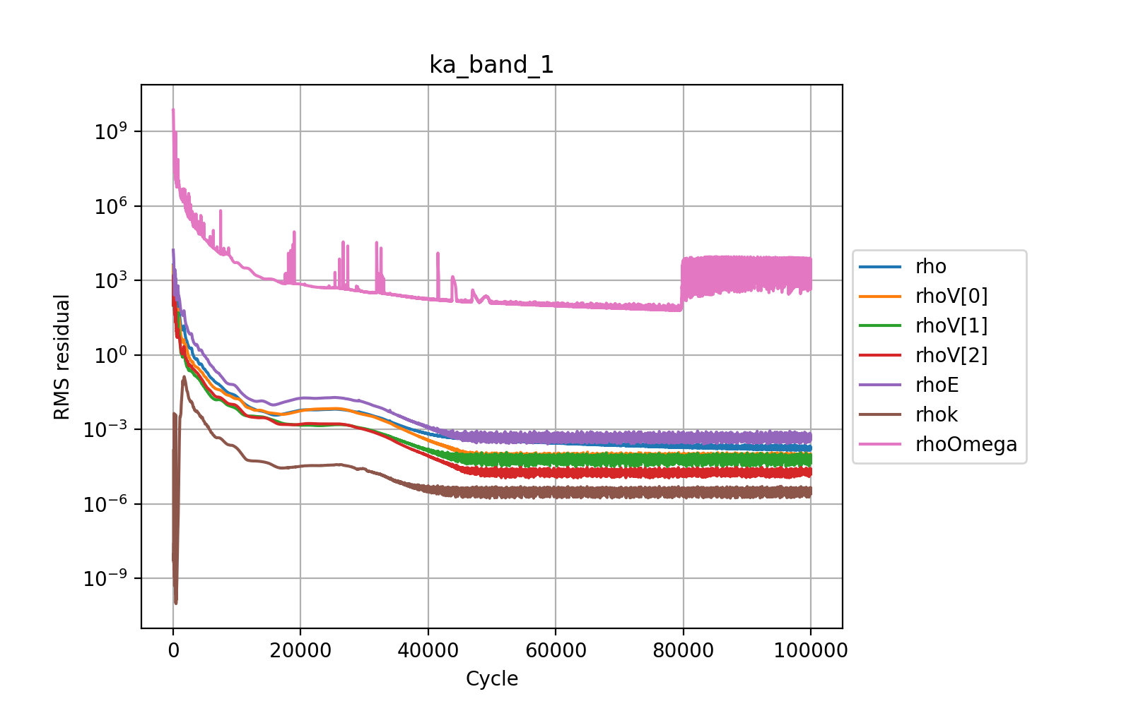
Fig. 7 The convergence of the steady-state explicit solver has achieved an average residual reduction of 5 orders of magnitude and then stalled. The noise in the solution from 40k cycles onwards suggests that either the flow is not fundamentally steady-state or that multigrid is adding an error to the solution. The user must determine whether the level of convergence is sufficient for their purposes and if not whether to run an unsteady simulation or degrade the spatial accuracy.
There are several common causes of convergence stall:
Multigrid
Flow unsteadiness
Multigrid
For explicit simulations, the use of multigrid will accelerate the convergence of the solver by using a set of coarse meshes to propagate longer wavelength solution components faster through the domain than would be possible on the finest mesh, subject to the CFL condition. In theory, and for idealised meshes, the use of multigrid does not change the steady-state solution (or pseudo-steady-state solution for unsteady flows) that is reached. However for real meshes around complex geometry, multigrid does introduce an error and this can effectively limit convergence. The use of the keyword ‘multigrid cycles’ in the ‘time marching’ section of the control dictionary will turn off multigrid after a specified number of cycles to remove this error.
Flow unsteadiness
A very common cause of convergence stall - particularly for steady-state simulations is due to physical unsteadiness in the underlying flow. In such cases, the solver is attempting to find a steady-state solution to an unsteady problem and the result is that the solution keeps changing in each iterative cycle. There are two approaches to dealing with this - depending upon the flow features of interest.
If the unsteadiness is important then the unconverged steady-state flow can be used as the starting point for an unsteady simulation. If the convergence stall is within the pseudo-steady cycles of an unsteady dual time-stepping solution, then it may be that the physical time step specified is too large and should be reduced.
On the other hand, if the unsteadiness is not of interest then the accuracy of the solution can be deliberately degraded to provide a more ‘average’ steady-state flow. This might include using the Rusanov inviscid flux scheme, switching the spatial accuracy to first order and / or using a coarser mesh. Note that the implicit mode of the solver can also be used to filter the solution in time as larger time-steps can be achieved with a higher CFL number. The user should note that this approach can cause solver instability and inaccuracy in the final solution, as the ‘averaging’ process is non-physical.
It may also be the case that the flow residuals are stalled, but the integrated properties of interest (e.g. lift, drag, mass flow) are sufficiently converged as to be useful. This decision is left to the user.