Tutorial 4: FWH Solver
A Ffowcs-Williams Hawkings (FWH) solver, which is used for prediction of farfield noise, is included in the zCFD distribution. In this section, we will use the zCFD FWH solver to calculate the sound experienced by two ‘observer microphones’ as a result of the aerodynamic noise generated by the flow around the cylinder.
In order to predict noise at observer microphone locations, an FWH solver requires an initial unsteady CFD solution. We will base our example on the CFD simulation setup from Tutorial 3 with some additional modifications to record the flow variables on an ‘FWH surface’ in the near-field, noise generating region. We then use the FWH solver to propagate the noise from the near-field FWH surface to the observer microphones.
The FWH solver can be run in two ways - the run_fwh utility and fwh python module. In this tutorial, the simpler run_fwh utility is introduced first, followed by the fwh python module and postprocessing using a jupyter notebook.
Running zCFD with FWH output
The flow we’re going to be running the FWH solver on is the shedding cylinder. To get the required inputs to our FWH solver, we need to define an FWH surface, and collect data on this surface during a CFD simulation.
The files required for the fwh tutorial can be downloaded here. In the zip file there’s a FWH surface definition file, called fwh_surface1.stl. Given we’ve already run the cylinder case in Tutorial 3, we can view the FWH surface in Paraview alongside the cylinder CFD volume data (see here), as below. You may find the surface easier to see if you set the view style to be Feature Edges instead of Surface for the FWH surface, and increase the Line Width in the Geometry Representation.
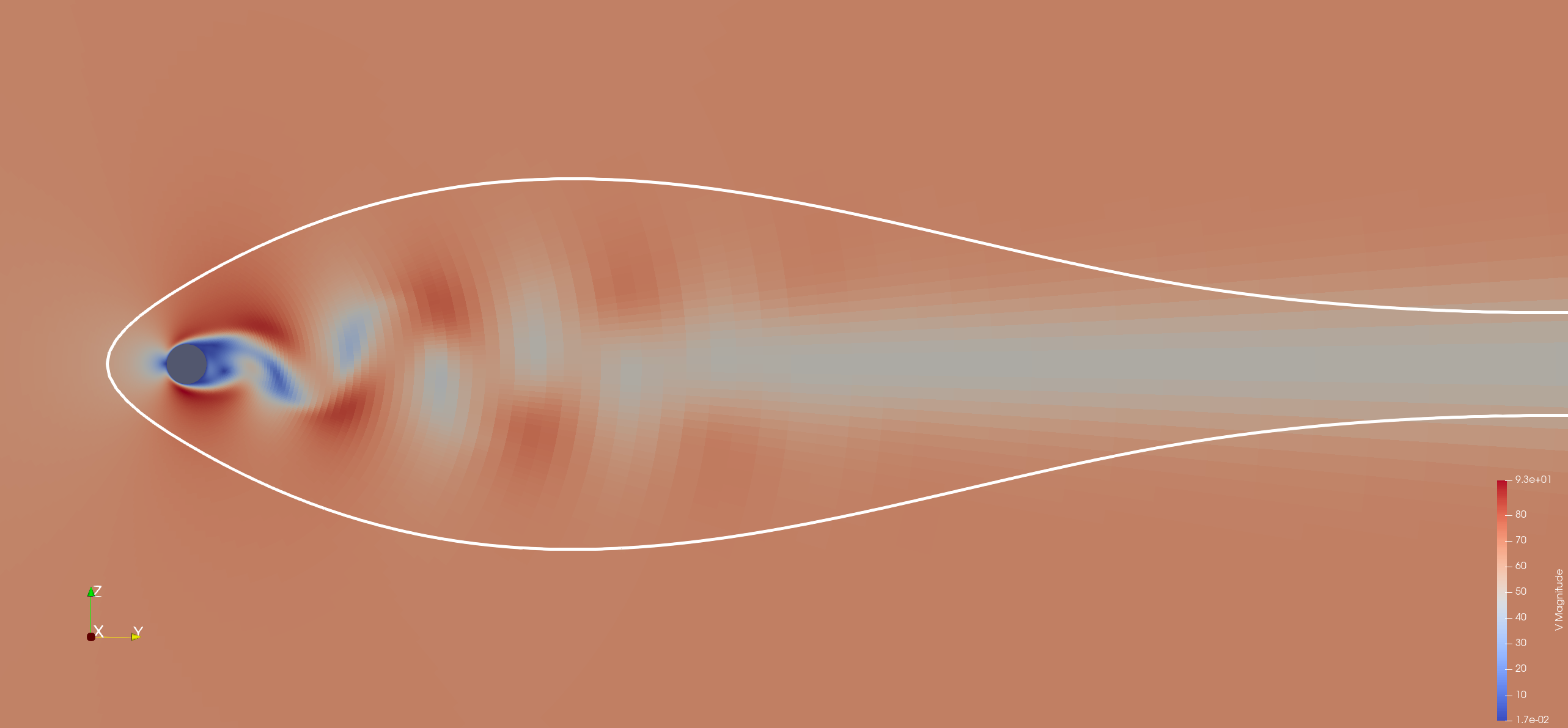
The FWH surface encloses the noise generating near-field region, but does not intersect the wake, in order to avoid spurious pseudo-sound [1, 2] .
There’s also a prepared control dictionary, cylinder_fwh.py. This is identical to tutorials 3’s cylinder.py apart from the output section, which is detailed below.
"write output": {
    "format": "vtk",
    "surface variables": ["V", "p", "T", "rho", "cp"],
    "volume variables": ["V", "p", "T", "rho", "m", "cp"],
    "fwh interpolate": ["fwh_surface1.stl"],
    "frequency": {
        "fwh interpolate": 1,
        "volume data": 1000,
        "surface data": 1000,
    },
},
In this case, we have chosen to output fwh interpolate data every single timestep, using the fwh_surface1.stl FWH surface definition file. Volume and surface data is much less frequent, since we already have all this data from when we ran cylinder.py above.
For the FWH tutorial we have also updated the ‘time marching’ section to run the simulation for 4 seconds, rather than 1.2. We run the CFD simulation in the normal way, using the command below.
run_zcfd -m cylinder.h5 -c cylinder_fwh.py
When we’ve run the CFD simulation of the cylinder, we should be able to see the FWH interpolated data in ‘cylinder_fwh_P1_OUTPUT/ACOUSTIC_DATA/fwh_surface1_FWHData.h5’. There is also a corresponding xdmf file, ‘cylinder_fwh_P1_OUTPUT/ACOUSTIC_DATA/fwh_surface1_FWHData.xdmf’, which allows us to open the FWH surface in Paraview and see the pressure, velocity and density at each cell centre varying with simulation time. Use the Paraview Time controls to adjust the simulation time being viewed. You may find that changing the view style to Point Gaussian and increasing the Gaussian Radius in the Properties sidebar makes the cell values easier to see.
Running the zCFD FWH solver
Using the run_fwh utility
We’re going to use the run_fwh utility to calculate noise at an observer Obs1. ‘Obs1’ is an observer that is a fixed distance away from the cylinder - if we consider the cylinder in a wind tunnel, we could consider ‘Obs1’ as a microphone attached to the wind tunnel wall. Since Obs1 is static relative to the FWH surface, it is in the same translational reference frame as the FWH surface and we can therefore use the run_fwh utility.

Fig. 1 FWH surface and Obs1 motions - CFD frame of reference
To use the run_fwh utility we need three inputs - a zCFD control file, a reference condition specification and an observers .csv file.
The zCFD control file is simply the control file for the zCFD simulation we used to create the FWH surface data - in this case, cylinder_fwh.py. run_fwh reads cylinder_fwh.py and can see that we have a single FWH surface, with data stored at ‘cylinder_fwh_P1_OUTPUT/ACOUSTIC_DATA/fwh_surface1_FWHData.h5’.
Next, we have to define a reference condition. In external flow simulations of this type, the run_fwh reference condition is the freestream conditions, defined as a zCFD IC block. In this case, the freestream conditions are already defined in cylinder_fwh.py to define the farfield boundary condition, so we can simply use ‘IC_1’ for the run_fwh reference condition.
Lastly, we need to define the name and location of our observers in a .csv file. The centre of the cylinder in the CFD mesh is at (0.25,0,0), and we want Obs1 to always be (0,0,20) metres away from the cylinder centre during the FWH simulation. The file Observers.csv (included in the tutorial .zip file) therefore contains the following:
Obs1, 0.25, 0.0, 20.0
Having decided on our inputs, we run the run_fwh utility by simply typing the following command within the zCFD command-line environment.
run_fwh -c cylinder_fwh.py --reference_condition IC_1 --observer_locations Observers.csv
Running this command prints output to screen and to the cylinder_fwh.fwh.log file, and outputs the FWH calculated pressure history at Obs1 to cylinder_fwh.fwh.Obs1.csv. In the case where there are multiple noise sources, the contribution of noise to each source is broken out, with the total observed noise also reported. Suggested post-processing is introduced below.
Using the fwh python module
As can be seen above, the run_fwh utility is very easy to use and is applicable in most simple FWH calculations. However, it has limitations - namely the fact that all observers and surfaces must be in the same translational reference frame, and that using it when more than one FWH surface encloses a noise generating region will lead to double accounting.
Where the run_fwh utility is not applicable, the fwh python module can be used instead. In this section, we will use the fwh python module to calculate observer pressure histories at both Obs1 and Obs2, where Obs2 is a ‘flyby’ observer whose pressure history cannot be calculated using the run_fwh utility.

Fig. 2 FWH surface and observer motions - CFD frame of reference
FWH Observer and surface motions
When the FWH equations are derived, we make an important assumption - that of a ‘quiescent medium’ (i.e. still air, with a free-stream velocity of zero). Clearly, with a freestream velocity of (0,66.8,0), the flow in our CFD simulation does not satisfy this condition. In order to use the FWH solver, we therefore have to perform a co-ordinate transformation, as in Fig. 3. In the run_fwh utility, this co-ordinate transformation is performed automatically, whereas in the fwh python module we set up the surface and observer motions through the FWH quiescent medium manually.
In this ‘quiescent medium’ co-ordinate system, the cylinder and ‘Obs1’ are ‘flying’ through the air. In this co-ordinate system, we can also see that ‘Obs2’ represents a microphone fixed to the ground, as the cylinder flies overhead.

Fig. 3 FWH surface and observer motions - FWH (quiescent medium) frame of reference
Setting up the FWH solver inputs
Now that we know the motions of our observers and surface, we can run the FWH solver. The python code required to run the FWH solver is in the file ‘run_fwh_solver.py’, and also written out below. We define the surfaces, observers and the solver settings, then use fwh.solve() to actually run the FWH solver.
from fwh import fwh, motion
import json
import math

# FWH surface motion
c  = math.sqrt(1.4 * 277.7777 * 287)
v_surf = [0, - 0.2 * c, 0] # = [0,-66.8,0]
surfaceCentrePoint = motion.ConstantVelocityPoint([0.0, 0.0, 0.0], v_surf)
surfaceMotion = motion.NonrotatingSurface(surfaceCentrePoint)

# obs1 motion - [0,0,20] above cylinder centre
obs1_CFD_frame_posn = [0.25,0,20]
obs1Motion = motion.ConstantVelocityPoint(obs1_CFD_frame_posn, v_surf)

# obs2 motion - stationary, intersects with obs1 at t=2.5
obs2_posn = []
for i in range(3):
  obs2_posn.append( obs1_CFD_frame_posn[i] + 2.5* v_surf[i])
obs2Motion = motion.StationaryPoint(obs2_posn)

solverSettings = {
    "c": c,
    "dt": 0.002,
    "rho0": 101325.0 / (277.7777 * 287),
    "p0": 101325.0,
}

surfaces = {
    "surf1": {
        "motion": surfaceMotion,
        "fileName": "./cylinder_fwh_P1_OUTPUT/ACOUSTIC_DATA/fwh_surface1_FWHData.h5",
    }
}
observers = {"Obs1": obs1Motion, "Obs2": obs2Motion}

pOut, tOut = fwh.solve(surfaces, observers, solverSettings)

dataForJson = {"p": pOut, "t": tOut}

with open("./FWH_data.json","w") as f:
    json.dump(dataForJson,f)
More details on FWH solver setup can be found here, but the most important concept is that we use ‘motion classes’ to define observer and surface motions. The available point (observer) motions are ‘OriginPoint’, ‘StationaryPoint’ and ‘ConstantVelocityPoint’. The available surface motions (which rely on a point motion to define the motion of their centre) are ‘NonrotatingSurface’ and ‘RotatingSurface’.
The velocities and fluid properties used in the FWH simulation are taken from the ‘cylinder.py’ zCFD control file. solverSettings['dt'] has been set to be the same as the timestep between outputs in the FWH surface data (0.002 seconds, see above).
In general, we can consider the motion of a point on an FWH surface to be defined by \(\mathbf{x}(t)=\mathbf{x}_0+ \mathbf{V}_{surf} \ t\) in the FWH co-ordinate frame. \(\mathbf{V}_{surf}\) is defined by the user in the surface motion class (called surfaceMotion above) and \(\mathbf{x}_0\) is the position defined by the FWH surface definition file (‘fwh_surface1.stl’, see above).
The centre of the cylinder in the CFD mesh is at (0.25,0,0), and we want Obs1 to always be (0,0,20) metres away from the cylinder centre during the FWH simulation. Since the cylinder ‘travels with’ the FWH surface (see Fig. 3), we can therefore say that the motion of the cylinder centre in the FWH co-ordinate frame is \(\mathbf{x}(t)=\left( (0.25,0,0) + (0,0,20) \right) + \mathbf{V}_{surf} t\). We therefore set the motion of Obs1 to be \(\mathbf{x}(t)= (0.25,0,20) + \mathbf{V}_{surf} t\). We set Obs2 to be stationary in the FWH reference frame, and to be coincident with Obs1 at t=2.5. We save the outputs to a json file called FWH_data.json.
Running the FWH solver
The python code above is replicated in ‘run_fwh_solver.py’. To run the FWH solver, we simply run the command below from within the zCFD command-line environment. You may need to change the surfaces["surf1"]["fileName"] parameter depending on how many ranks you used in your zCFD run.
python3 run_fwh_solver.py
This will output various information to the screen, including the ‘valid min and max times’ for each surface / observer combination.
The valid min and max times denote the time window during which an observer receives data from all points on the FWH surface. A pressure signal emitted from a point on the FWH surface at time t takes r/c seconds to arrive at an observer, where r is the distance from the surface point to observer and c is the speed of sound. Therefore the valid observer time window will always be later than the FWH surface output time window (in our case, 0.002:1.2 seconds) due to the distance from the FWH surface to the observer. The valid observer time window will be narrower if the FWH surface is large, since the larger the surface the larger the time delay between signals from different points on the surface reaching the observer becomes.
Post-processing
The jupyter notebook postprocess_fwh_module_data.ipynb from the .zip file can be used to post-process the FWH data. postprocess_fwh_module_data.ipynb uses the data from the fwh python module section of this tutorial, but an equivalent notebook which uses the data from the run_fwh utility section is available in postprocess_run_fwh_data.ipynb.
These notebooks contain a number of zutil functions which may be useful for users wishing to perform acoustic post-processing. The notebooks plot the pressure history p(t) and power spectral density (PSD) at both observers, as below.
Obs1 moves through the FWH medium at a constant displacement from the cylinder centre (see Fig. 3). We see from our post-processing that the noise experienced by Obs1 is dominated by a constant 10 Hz component, which is the shedding frequency of the cylinder. Various harmonics of the 10 Hz signal are present in the power spectral density plot for Obs1.


During the FWH simulation run in the fwh python module section of this tutorial, the cylinder gets closer to Obs2 from 0 to 2.5 seconds, before getting further away from Obs2 from 2.5 seconds onwards. We can see in the Obs2 p(t) plot that the peaks are closer together from 0 to 2.5 seconds than they are after 2.5 seconds. This is due to Doppler shift. We can also see the effect of Doppler shift in the power spectral density, which has a more rounded 10 Hz peak than that seen in Obs1.


postprocess_fwh_module_data.ipynb also creates .wav files, which allow you to listen to the sound experienced by Obs1 and Obs2.
Extensions
To become more comfortable with the FWH solver, various extensions to this exercise are possible. Here are some suggestions.
Re-run the zCFD solver, but this time extract FWH data on the cylinder wall instead of fwh_surface1.stl. Run the FWH solver (using the wall data as an impermeable FWH surface) and compare the results to those achieved using the fwh_surface1 permeable FWH surface.
Re-run the zCFD solver, but this time also extract FWH data on the fwh_surface2.stl and fwh_surface3.stl surfaces. These are like fwh_surface1.stl but slightly larger. Run the FWH solver with these surfaces and investigate the effect of using different surfaces on the FWH results. You will have to do this using the fwh python module to avoid double accounting.
Add extra observers of your choice to the FWH solver.
Use the file utility writeFWHSurfaceFrequenciesFile to visually inspect the spatial distribution of different frequencies in the FWH surface.
Use the file utility writeBlankedOffFwhSurfaceFile to ‘blank off’ all FWH surface cells more than 5 cylinder diameters downstream of the cylinder’s centre. Run the FWH solver using this modified surface, and based on this estimate how much of the shedding noise originates more than 5 diameters downstream of the cylinder.
Use the solver.fwh_helper_functions module to rewrite run_fwh_solver.py so that the solverSettings dictionary is automatically set based on the zCFD control file name and reference condition which were used in the run_fwh utility.
Note
Since the cylinder CFD simulation is ‘2.5D’ (i.e. the mesh only has a single cell in the x direction), the distance scaling of p(t) at observers will be non-physical.
Citations
Mitchell, B., Lele, S., & Moin, P. (1999). Direct computation of the sound generated by vortex pairing in an axisymmetric jet. Journal of Fluid Mechanics, 383, 113-142. 10.1017/S0022112099003869
Ricciardi, T. R. , Wolf W. R, & Spalart P. R. (2022). On the Application of Incomplete Ffowcs Williams and Hawkings Surfaces for Aeroacoustic Predictions. AIAA Journal, 60:3, 1971-1977. 10.2514/1.J061285